LambdaLisp - A Lisp Interpreter That Runs on Lambda Calculus

LambdaLisp is a Lisp interpreter written as an untyped lambda calculus term. The input and output text is encoded into closed lambda terms using the Mogensen-Scott encoding, so the entire computation process solely consists of the beta-reduction of lambda calculus terms.

When run on a lambda calculus interpreter that runs on the terminal, it presents a REPL where you can interactively define and evaluate Lisp expressions. Supported interpreters are:

• The 521-byte lambda calculus interpreter SectorLambda written by Justine Tunney
• The IOCCC 2012 “Most functional” interpreter written by John Tromp (the source is in the shape of a λ)
• Universal Lambda interpreter clamb and Lazy K interpreter lazyk written by Kunihiko Sakamoto

Supported features are:

• Signed 32-bit integers
• Strings
• Closures, lexical scopes, and persistent bindings with let
• Object-oriented programming feature with class inheritance
• Reader macros with set-macro-character
• Access to the interpreter’s virtual heap memory with malloc, memread, and memwrite
• Show the call stack trace when an error is invoked
• Garbage collection during macro evaluation

and much more.

LambdaLisp can be used to write interactive programs. Execution speed is fast as well, and the number guessing game runs on the terminal with an almost instantaneous response speed.

Here is a PDF showing its entire lambda term, which is 42 pages long:

The embedded PDF may not show on mobile. The same PDF is also available at https://woodrush.github.io/lambdalisp.pdf.

Page 32 is particulary interesting, consisting entirely of (s:

Overview

LambdaLisp is a Lisp interpreter written as a closed untyped lambda calculus term. It is written as a lambda calculus term ${\rm LambdaLisp} = \lambda x. \cdots$ which takes a string $x$ as an input and returns a string as an output. The input $x$ is the Lisp program and the user’s standard input, and the output is the standard output. Characters are encoded into lambda term representations of natural numbers using the Church encoding, and strings are encoded as a list of characters with lists expressed as lambdas in the Mogensen-Scott encoding, so the entire computation process solely consists of the beta-reduction of lambda terms, without introducing any non-lambda-type object. In this sense, LambdaLisp operates on a “truly purely functional language” without any primitive data types except for lambda terms.

Supported features are closures and persistent bindings with let, reader macros, 32-bit signed integers, a built-in object-oriented programming feature based on closures, and much more. LambdaLisp is tested by running code on both Common Lisp and LambdaLisp and comparing their outputs. The largest LambdaLisp-Common-Lisp polyglot program that has been tested is lambdacraft.cl, which runs the Lisp-to-lambda-calculus compiler LambdaCraft I wrote for this project, also used to compile LambdaLisp itself.

When run on a lambda calculus interpreter that runs on the terminal, LambdaLisp presents a REPL where you can interactively define and evaluate Lisp expressions. These interpreters automatically process the string-to-lambda encoding for handling I/O through the terminal.

Lisp has been described by Alan Kay as the Maxwell’s equations of software. In the same sense, I believe that lambda calculus is the particle physics of computation. LambdaLisp may therefore be a gigantic electromagnetic Lagrangian that connects the realm of human-friendly programming to the origins of the notion of computation itself.

Usage

LambdaLisp is available on GitHub at https://github.com/woodrush/lambdalisp. Here we will explain how to try LambdaLisp right away on x86-64-Linux and other platforms such as Mac.

Running the LambdaLisp REPL (on x86-64-Linux)

You can try the LambdaLisp REPL on x86-64-Linux by simply running:

git clone https://github.com/woodrush/lambdalisp
cd lambdalisp
make run-repl

The requirement is cc which should be installed by default. To try it on a Mac, please see the next section.

This will run LambdaLisp on SectorLambda, the 521-byte lambda calculus interpreter. The source code being run is lambdalisp.blc, which is the lambda calculus term shown in lambdalisp.pdf written in binary lambda calculus notation.

SectorLambda automatically takes care of the string-to-lambda I/O encoding to run LambdaLisp on the terminal. Interaction is done by writing LambdaLisp in continuation-passing style, allowing a Haskell-style interactive I/O to work on lambda calculus interpreters.

When building SectorLambda, Make runs the following commands to get its source codes:

• Blc.S: wget https://justine.lol/lambda/Blc.S?v=2
• flat.lds: wget https://justine.lol/lambda/flat.lds

After running make run-repl, the REPL can also be run as:

( cat ./bin/lambdalisp.blc | ./bin/asc2bin; cat ) | ./bin/Blc

Running the LambdaLisp REPL (on Other Platforms)

SectorLambda is x86-64-Linux exclusive. On other platforms such as a Mac, the following command can be used:

git clone https://github.com/woodrush/lambdalisp
cd lambdalisp
make run-repl-ulamb

This runs LambdaLisp on the lambda calculus interpreter clamb. The requirement for this is gcc or cc.

After running make run-repl-ulamb, the REPL can also be run as:

( cat ./bin/lambdalisp.ulamb | ./bin/asc2bin; cat ) | ./bin/clamb -u

LambdaLisp supports other various lambda calculus interpreters as well. For instructions for other interpreters, please see the GitHub repo.

Playing the Number Guessing Game

Once make run-repl is run, you can play the number guessing game with:

( cat ./bin/lambdalisp.blc | ./bin/asc2bin; cat ./examples/number-guessing-game.cl; cat ) | ./bin/Blc

If you ran make run-repl-ulamb, you can run:

( cat ./bin/lambdalisp.ulamb | ./bin/asc2bin; cat ./examples/number-guessing-game.cl; cat ) | ./bin/clamb -u

You can run the same script on Common Lisp. If you use SBCL, you can run it with:

sbcl --script ./examples/number-guessing-game.cl

Examples

Closures

The following LambdaLisp code runs right out of the box:

(defun new-counter (init)
  ;; Return a closure.
  ;; Use the let over lambda technique for creating independent and persistent variables.
  (let ((i init))
    (lambda () (setq i (+ 1 i)))))

;; Instantiate counters
(setq counter1 (new-counter 0))
(setq counter2 (new-counter 10))

(print (counter1)) ;; => 1
(print (counter1)) ;; => 2
(print (counter2)) ;; => 11
(print (counter1)) ;; => 3
(print (counter2)) ;; => 12
(print (counter1)) ;; => 4
(print (counter1)) ;; => 5

An equivalent JavaScript code is:

// Runs on the browser's console
function new_counter (init) {
    let i = init;
    return function () {
        return ++i;
    }
}

var counter1 = new_counter(0);
var counter2 = new_counter(10);

console.log(counter1()); // => 1
console.log(counter1()); // => 2
console.log(counter2()); // => 11
console.log(counter1()); // => 3
console.log(counter2()); // => 12
console.log(counter1()); // => 4
console.log(counter1()); // => 5

Object-Oriented Programming With Class Inheritance

As described in Let Over Lambda, when you have closures, you get object-oriented programming for free. LambdaLisp has a built-in OOP feature implemented as predefined macros based on closures. It supports Python-like classes with class inheritance:

;; Runs on LambdaLisp
(defclass Counter ()
  (i 0)

  (defmethod inc ()
    (setf (. self i) (+ 1 (. self i))))

  (defmethod dec ()
    (setf (. self i) (- (. self i) 1))))


(defclass Counter-add (Counter)
  (defmethod *init (i)
    (setf (. self i) i))

  (defmethod add (n)
    (setf (. self i) (+ (. self i) n))))


(defparameter counter1 (new Counter))
(defparameter counter2 (new Counter-add 100))

((. counter1 inc))
((. counter2 add) 100)

(setf (. counter1 i) 5)
(setf (. counter2 i) 500)

An equivalent Python code is:

class Counter ():
    i = 0

    def inc (self):
        self.i += 1
        return self.i
    
    def dec (self):
        self.i -= 1
        return self.i

class Counter_add (Counter):
    def __init__ (self, i):
        self.i = i
    
    def add (self, n):
        self.i += n
        return self.i

counter1 = Counter()
counter2 = Counter_add(100)

counter1.inc()
counter2.add(100)

counter1.i = 5
counter2.i = 500

More Examples

More examples can be found in the GitHub repo. The largest LambdaLisp program currently written is lambdacraft.cl, which runs the lambda calculus compiler LambdaCraft I wrote for this project, also used to compile LambdaLisp itself.

Features

Key features are:

• Signed 32-bit integers
• Strings
• Closures, lexical scopes, and persistent bindings with let
• Object-oriented programming feature with class inheritance
• Reader macros with set-macro-character
• Access to the interpreter’s virtual heap memory with malloc, memread, and memwrite
• Show the call stack trace when an error is invoked
• Garbage collection during macro evaluation

Supported special forms and functions are:

• defun, defmacro, lambda (&rest can be used)
• quote, atom, car, cdr, cons, eq
• +, -, *, /, mod, =, >, <, >=, <=, integerp
• read (reads Lisp expressions), print, format (supports ~a and ~%), write-to-string, intern, stringp
• let, let*, labels, setq, boundp
• progn, loop, block, return, return-from, if, cond, error
• list, append, reverse, length, position, mapcar
• make-hash-table, gethash (setf can be used)
• equal, and, or, not
• eval, apply
• set-macro-character, peek-char, read-char, ` , ,@ ' #\
• carstr, cdrstr, str, string comparison with =, >, <, >=, <=, string concatenation with +
• defun-local, defglobal, type, macro
• malloc, memread, memwrite
• new, defclass, defmethod, ., field assignment by setf

Tests

There are 2 types of tests written for LambdaLisp. The GitHub Actions CI runs these tests.

Output Comparison Test

The files examples/*.cl run both on Common Lisp and LambdaLisp producing identical results, except for the initial >   printed by the REPL in LambdaLisp. This test first runs *.cl on both SBCL and LambdaLisp and compares their outputs.

The files examples/*.lisp are LambdaLisp-exclusive programs. The output of these files are compared with test/*.lisp.out.

LambdaCraft Compiler Hosting Test

examples/lambdacraft.cl runs LambdaCraft, a Common-Lisp-to-lambda-calculus compiler written in Common Lisp, used to compile the lambda calculus source for LambdaLisp. The script defines a binary lambda calculus (BLC) program that prints the letter A and exits, and prints the BLC source code for the defined program.

The LambdaCraft compiler hosting test first executes examples/lambdacraft.cl on LambdaLisp, then runs the output BLC program on a BLC interpreter, and checks if it prints the letter A and exits.

Experimental: Self-Hosting Test

This test is currently theoretical since it requires a lot of time and memory, and is unused in make test-all. This test extends the previous LambdaCraft compiler hosting test and checks if the Common Lisp source code for LambdaLisp runs on LambdaLisp itself. Since the LambdaCraft compiler hosting test runs properly, this test should theoretically run as well, although it requires a tremendous amount of memory and time. The test is run on the binary lambda calculus interpreter Blc.

One concern is whether the 32-bit heap address space used internally in LambdaLisp is enough to compile this program. This can be solved by compiling LambdaLisp with an address space of 64-bit or larger, which can be done simply by replacing the literal 32 (which only appears once in src/lambdalisp.cl) with 64, etc. Another concern is whether if the execution hits Blc’s maximum term limit. This can be solved by compiling Blc with a larger memory limit, by editing the rule for $(BLC) in the Makefile.

How it Works - LambdaLisp Implementation Details

Here we will explain LambdaLisp’s implementation details. Below is a table of contents:

• General Lambda Calculus Programming
  • Handling I/O in Lambda Calculus
  • Lambda-Calculus-Based Programming Languages
  • Lazy K
  • Interactive I/O in Lambda-Calculus-Based Languages
• LambdaLisp Implementation Details
  • The Core Implementation Strategy
  • The Startup Phase - A Primitive Form of Asynchronous Programming
  • The Basic Evaluation Loop
  • Basic Data Structures
  • Virtual Heap Memory (RAM)
  • Registers (Global Variables)
  • The Prelude Generator and String Compression
• Language Features
  • The Memory Model for Persistent Bindings
  • Garbage Collection
  • Macros
  • Object-Oriented Programming
  • Blocks
  • Loops
  • Error Invocation and Stack Traces
• Other General Lambda Calculus Programming Techniques
  • Mutual Recursion
  • Deriving ‘isnil’
  • LambdaCraft’s ‘do’ Macro
  • Print Debugging
  • Type Checking with Macro Call Signatures
• Appendix
  • JavaScript Examples of Continuation-Passing Style Code
  • The Binary Lambda Calculus Notation
• About the Logo
• Credits

General Lambda Calculus Programming

Before introducing LambdaLisp-specific implementation details, we’ll cover some general topics about programming in lambda calculus.

Handling I/O in Lambda Calculus

LambdaLisp is written as a function ${\rm LambdaLisp} = \lambda x. \cdots$ which takes one string as an input and returns one string as an output. The input represents the Lisp program and the user’s standard input (the $x$ is the input string), and the output represents the standard output. A string is represented as a list of bits of its ASCII representation. In untyped lambda calculus, a method called the Mogensen-Scott encoding can be used to express a list of lambda terms as a pure untyped lambda calculus term, without the help of introducing a non-lambda-type object.

Bits are encoded as:

$$\begin{aligned} 0 &= \lambda x. \lambda y. x \\ 1 &= \lambda x. \lambda y. y \\ \end{aligned}$$

Lists are made using the list constructor and terminator ${\rm cons}$ and ${\rm nil}$:

$$\begin{aligned} {\rm cons} &= \lambda x. \lambda y. \lambda f. (f x y) \\ {\rm nil} &= \lambda x. \lambda y. y \end{aligned}$$

Note that $1 = {\rm nil}$. Under these rules, the bit sequence 0101 can be expressed as a composition of lambda terms:

$$({\rm cons} ~ 0 ~ ({\rm cons} ~ 1 ~ ({\rm cons} ~ 0 ~ ({\rm cons} ~ 1 ~ {\rm nil}))))$$

which is exactly the same as how lists are constructed in Lisp. This beta-reduces to:

$$\begin{aligned} \lambda f. &(f (\lambda x.\lambda y.x) \lambda g.(g (\lambda x.\lambda y.y) \\ &\lambda h.(h (\lambda x.\lambda y.x) \lambda i.(i (\lambda x.\lambda y.y) (\lambda x.\lambda y.y))))) \end{aligned}$$

Using this method, both the standard input and output strings can entirely be encoded into pure lambda calculus terms, letting LambdaLisp to operate with beta reduction of lambda terms as its sole rule of computation, without the requirement of introducing any non-lambda-type object.

The LambdaLisp execution flow is thus as follows: you first encode the input string (Lisp program and stdin) as lambda terms, apply it to ${\rm LambdaLisp} = \lambda x. \cdots$, beta-reduce it until it is in beta normal form, and parse the output lambda term as a Mogensen-Scott-encoded list of bits (inspecting the equivalence of lambda terms is quite simple in this case since it is in beta normal form). This rather complex flow is supported exactly as is in 3 lambda-calculus-based programming languages: Binary Lambda Calculus, Universal Lambda, and Lazy K.

Lambda-Calculus-Based Programming Languages

Binary Lambda Calculus (BLC) and Universal Lambda (UL) are programming languages with the exact same I/O strategy described above - a program is expressed as one pure lambda term that takes a Church-Mogensen-Scott-encoded string and returns a Church-Mogensen-Scott-encoded string. When the interpreters for these languages Blc and clamb are run on the terminal, the interpreter automatically encodes the input bytestream to lambda terms, performs beta-reduction, parses the output lambda term as a list of bits, and prints the output as a string in the terminal.

The differences in BLC and UL are in a slight difference in the method for encoding the I/O. Otherwise, both of these languages follow the same principle, where lambda terms are the solely available object types in the language.

In BLC and UL, lambda terms are written in a notation called binary lambda calculus. Details on the BLC notation is described in the Appendix.

Lazy K

Lazy K is a language with the same I/O strategy with BLC and UL except programs are written as SKI combinator calculus terms instead of lambda terms. The SKI combinator calculus is a system equivalent to lambda calculus, where there are only 3 functions:

$$\begin{aligned} S &= \lambda x.\lambda y.\lambda z.(x z (y z)) \\ K &= \lambda x.\lambda y.x \\ I &= \lambda x.x \end{aligned}$$

Every SKI combinator calculus term is written as a combination of these 3 functions.

Every SKI term can be easily be converted to an equivalent lambda calculus term by simply rewriting the term with these rules. Very interestingly, there is a method for converting the other way around - there is a consistent method to convert an arbitrary lambda term with an arbitrary number of variables to an equivalent SKI combinator calculus term. This equivalence relation with lambda calculus proves that SKI combinator calculus is Turing-complete.

Apart from the strong condition that only 3 predefined functions exist, the beta-reduction rules for the SKI combinator calculus are exactly identical as that of lambda calculus, so the computation flow and the I/O strategy for Lazy K is the same as BLC and Universal Lambda - all programs can be written purely in SKI combinator calculus terms without the need of introducing any function other than S, K, and I. This allows Lazy K’s syntax to be astonishingly simple, where only 4 keywords exist - s, k, i, and ` for function application.

As mentioned in the original Lazy K design proposal, if BF captures the distilled essence of structured imperative programming, Lazy K captures the distilled essence of functional programming. It might as well be the assembly language of lazily evaluated functional programming. With the simple syntax and rules orchestrating a Turing-complete language, I find Lazy K to be a very beautiful language being one of my all-time favorites.

LambdaLisp is written in these 3 languages - Binary Lambda Calculus, Universal Lambda, and Lazy K. In each of these languages, LambdaLisp is expressed as one lambda term or SKI combinator calculus term. Therefore, to run LambdaLisp, an interpreter for one of these languages is required. To put in a rather convoluted way, LambdaLisp is a Lisp interpreter that runs on another language’s interpreter.

Interactive I/O in Lambda-Calculus-Based Languages

The I/O model described previously looks static - at first sight it seems as if the entire value of ${\rm stdin}$ needs to be pre-supplied beforehand on execution, making interactive programs be impossible. However, this is not the case. The interpreter handles interactive I/O by the following clever combination of input buffering and lazy evaluation:

• The input string is buffered into the memory. Its values are lazily evaluated - execution proceeds until the last moment an input needs to be referenced in order for beta reduction to proceed.

• The output string is printed as soon as the interpreter deduces the first characters of the output string.

As an example, consider the BLC program ${\rm ROT13}$ which initially prints a prompt In>, accepts standard input, then outputs the ROT13 encoding of the standard input. After the user starts the program, the interpreter’s beta-reduction proceeds as follows:

$$\begin{aligned} {\rm ROT13} ~ {\rm stdin} &= (\lambda s.{\rm Code} ~ s) ~ {\rm stdin} \\ &= ({\rm Code} ~ {\rm stdin}) \\ &= ({\rm cons} ~ \tilde I ~ ({\rm Code}_1 ~ {\rm stdin})) \\ &= ({\rm cons} ~ \tilde I ~ ({\rm cons} ~ \tilde n ~ ({\rm Code}_2 ~ {\rm stdin}))) \\ &= ({\rm cons} ~ \tilde I ~ ({\rm cons} ~ \tilde n ~ ({\rm cons} ~ \tilde > ~ ({\rm Code}_3 ~ {\rm stdin})))) \\ \end{aligned}$$

Here, $\tilde I$ is a lambda term representing the character I.

As ${\rm Code}$ is beta-reduced, it “weaves out” its output string In> on the way. This is somewhat akin to the central dogma of molecular biology, where ribosomes transcribe genetic information to polypeptide chains - the program is the gene, the interpreter is the ribosome, and the list of output characters is the polypeptide chain.

The interpreter continues its evaluation until further beta reduction is impossible without the knowledge of the value of ${\rm stdin}$, which happens at ${\rm Code}_3$. At this point, the string In> is shown on the terminal since its values are already determined and available.

Seeing the prompt In>, suppose that the user types the string “Hi”. The interpreter then buffers its lambda-encoded expression into the pointer that points to ${\rm stdin}$, making the evaluation proceed as:

$$\begin{aligned} r.h.s. &= ({\rm cons} ~ \tilde I ~ ({\rm cons} ~ \tilde n ~ ({\rm cons} ~ \tilde > ~ ({\rm cons} ~ \tilde U ~ ({\rm Code}_4 ~ {\rm stdin}))))) \\ &= ({\rm cons} ~ \tilde I ~ ({\rm cons} ~ \tilde n ~ ({\rm cons} ~ \tilde > ~ ({\rm cons} ~ \tilde U ~ ({\rm cons} ~ \tilde v ~ ({\rm Code}_5 ~ {\rm stdin})))))) \\ \end{aligned}$$

On the terminal, the interaction process would look like this:

In>[**Halts; User types string**]Hi[**User types return; `Hi` is buffered into stdin**]
Uv

LambdaLisp Implementation Details

We will now cover LambdaLisp-specific implementation details.

The Core Implementation Strategy

When viewed as a programming language, lambda calculus is a purely functional language. This derives the following two basic programming strategies for LambdaLisp:

• In order to use global variables, the global state is passed to every function that affects or relies on the global state.
• In order to control the evaluation flow for I/O, continuation-passing style (CPS) is used.

Writing in continuation-passing style also helps the lambda calculus interpreter to prevent re-evaluating the same term multiple times. This is very, very important and critical when writing programs for the 521-byte binary lambda calculus interpreters Blc, tromp and uni, since it seems that they lack a memoization feature, although they readily have a garbage collection feature. Writing in direct style gradually slows down the runtime execution speed since memoization does not occur and the same computation is repeated multiple times. However, by carefully writing the entire program in continuation-passing style, the evaluation flow can be controlled so that the program only proceeds when the value under attention is in beta-normal form. In this situation, since values are already evaluated to their final form, the need for memoization becomes unnecessary in the first place.

The continuation-passing style technique suddenly transforms Blc to a very, very fast and efficient lambda calculus interpreter. In fact, the largest program lambdacraft.cl runs the fastest and even the most memory-efficient on Blc, using only about 1.7 GB of memory, while clamb uses about 5GB of memory. I suspect that the speed is due to a efficient memory configuration and the memory efficiency is due to the garbage collection feature. I was very surprised how large of a galaxy is fit into the microcosmos of 521 bytes! This realization that continuation-passing-style programs run very fast on Blc was what made everything possible and what motivated me to set on the journey of building LambdaCraft and LambdaLisp.

The difference between continuation-passing style and direct style is explained in the Appendix, with JavaScript code samples that run on the browser’s console.

The Startup Phase - A Primitive Form of Asynchronous Programming

Right after LambdaLisp starts running, it runs the following steps:

• The string generator decompresses the “prelude Lisp code”, and also generates keyword strings such as quote.
• The initial prompt carret >   is printed.
• The prelude Lisp code is silently evaluated (the results are not printed).
• The user’s initial input is evaluated and the results are printed.
• The interpreter enters the basic read-eval-print-loop.

The prelude Lisp code is a LambdaLisp code that defines core functions such as defun and defmacro as macros. The prelude is hard-coded as a compressed string, which is decompressed by the string generator before being passed to the interpreter. The compression method is described later. The LambdaLisp core code written in LambdaCraft hard-codes only the essential and speed-critical functions. Other non-critical functions are defined through LambdaLisp code in the prelude. A lot of the features including defun and defmacro which seem to look like keywords are in fact defined as macros. Due to this implementation, it is in fact possible to override the definition of defun to something else using setq, but I consider that as a flexible feature.

There is in fact a subtle form of asynchronous programming in action in this startup phase. Since the prelude code takes a little bit of time to evaluate since it contains a lot of code, if the initial prompt carret > is shown after evaluating the prelude code, it causes a slightly stressful short lag until the prelude finishes running.

To circumvent this, the the initial prompt carret > is printed before the prelude is loaded. This allows the prelude code to be evaluated while the user is typing their initial Lisp code. Since the input is buffered in all of the lambda calculus interpreters, their input does not get lost even when the prelude is running in the background. If the user types very fast, there will become a little bit of waiting until the result of the inital input is shown, but if the prelude is already loaded, their result will be shown right away. All later inputs are evaluated faster because the prelude is only read once at initialization. In a way, this is a primitive form of asynchronous programming, where processing the user input and the execution of some code is done concurrently.

The Basic Evaluation Loop

After the prelude is loaded, the interpreter enters its basic read-eval-print loop.

As mentioned before, the basic design is that all state-affecting functions must pass the state as arguments, and basicallly all functions are written in CPS. This makes the core eval function have the following signature:

;; LambdaCraft
(defrec-lazy eval (expr state cont)
  ...)

Where expr is a Lisp expression, state is the global state, and cont is the continuation. The comment ;; LambdaCraft indicates that this is the source code for the LambdaLisp interpreter written in LambdaCraft.

The direct return type of eval is string, and not expr or state. This is because the entire program is expected to be a program that “takes a string and outputs a string”. This design also allows print debugging to be written very intuitively in an imperative style as discussed later.

Instead of using the direct return values, the evaluation results are “returned” to later processes through the continuation cont. cont is actually just a callback function that is called at the end of eval, which is called with the evaluated expr and the new state as its arguments. For example, if the evaluation result is 42 and the renewed state is state, eval calls the callback function cont as

(cont result state) ;; Where result == 42 and state is the renewed state

in the final step of the code. Here, two values result and state are “returned” to the callback function cont and are used later in cont.

Having the direct return type of eval to be a string makes the implementation of exit very simple. It is implemented in eval as:

;; LambdaCraft
((stringeq (valueof head) kExit)
  nil)

Here is how it works:

• Normally, every successive chain of computations is evoked by calling the callback function (the continuation). Here, since eval no longer calls a continuation when exit is called, no further computation happens and the interpreter stops there.
• eval’s direct return value is set to nil, which is a string terminator. This leaves nil at the end of the output string, completing the value of the output string.

A similar implementation is used for read-expr, which exits the interpreter when there is no more text to read:

;; LambdaCraft
;; Exit the program when EOF is reached
(if (isnil stdin)
  nil)

Basic Data Structures

The state is a 3-tuple that contains reg, heap and stdin. In lambda terms:

$$\begin{aligned} {\rm state} &:= {\rm cons3} ~ {\rm reg} ~ {\rm heap} ~ {\rm stdin} \\ &= (\lambda a. \lambda b. \lambda c. \lambda f. (f~a~b~c)) ~ {\rm reg} ~ {\rm heap} ~ {\rm stdin} \\ &= \lambda f. ~ (f ~ {\rm reg} ~ {\rm heap} ~ {\rm stdin}) \end{aligned}$$

reg is used to store values of global variables used internally by the interpreter. heap is a virtual heap memory used to store the let and lambda bindings caused by the code. stdin is the pointer to the standard input provided by the interpreter.

Similar with cons, state is a function that accepts a callback function and applies it with the values it’s storing. Therefore, the contents of state can be extracted by passing a callback function to state:

;; LambdaCraft
(state
  (lambda (reg heap stdin)
    [do something with reg/heap/stdin]))

which is continuation-passing style code, since we are using callback functions that accept values and describes what to do with those values.

expr is a Lisp expression. Expressions in LambdaLisp belong to one of the following 5 types: atom, cons, lambda, integer, and string. All expressions are a 2-tuple with a type tag and its value:

$${\rm expr} = {\rm cons} ~ {\rm typetag} ~ {\rm value} = \lambda f. ~ (f ~ {\rm typetag} ~ {\rm value})$$

The structure of ${\rm value}$ depends on the type. For all types, ${\rm typetag}$ is a selector for a 5-tuple:

$$\begin{aligned} {\rm type\_ atom} &= \lambda a.\lambda b.\lambda c.\lambda d.\lambda e. a \\ {\rm type\_ cons} &= \lambda a.\lambda b.\lambda c.\lambda d.\lambda e. b \\ {\rm type\_ lambda} &= \lambda a.\lambda b.\lambda c.\lambda d.\lambda e. c \\ {\rm type\_ integer} &= \lambda a.\lambda b.\lambda c.\lambda d.\lambda e. d \\ {\rm type\_ string} &= \lambda a.\lambda b.\lambda c.\lambda d.\lambda e. e \\ \end{aligned}$$

This way, we can do type matching by writing:

(typetag
  [code for atom case]
  [code for cons case]
  [code for lambda case]
  [code for integer case]
  [code for string case])

Type matching ensures that the ${\rm value}$ for each type is always processed correctly according to its type. Since each tag is a selector of a 5-tuple, the tag will select the code that will be executed next. Since all codes are lazily evaluated, the codes for the unselected cases will not be evaluated.

As in the case of state, the type and value can be extracted by passing a callback to expr:

;; LambdaCraft
(expr
  (lambda (dtype value)
    (dtype
      [do something with `value`])))

Virtual Heap Memory (RAM)

The virtual heap memory (RAM) is expressed as a binary tree constructed by the tuple constructor cons. The idea of using a binary tree data structure for expressing a RAM unit is borrowed from irori’s Unlambda VM (in Japanese). The implementation of the binary tree is modified from this definition so that the tree could be initialized as nil.

One RAM cell can store a value of any size and any type - Lisp terms, strings, or even the interpreter’s current continuation. This is because the RAM can actually only store one type, lambdas, but everything in lambda calculus belongs to that one type.

Trees are constructed using the same constructor ${\rm cons} = \lambda x. \lambda y. \lambda f. (f x y)$ as lists. A list $L$ containing A B C can be written using ${\rm cons}$ as:

$$L = ({\rm cons} ~ A ~ ({\rm cons} ~ B ~ (\rm cons ~ C ~ {\rm nil})))$$

Using the same mechanism, the following binary tree $T$,

can be expressed using ${\rm cons}$ cells as follows:

$$T = ({\rm cons} ~ ({\rm cons} ~ A ~ B) ~ ({\rm cons} ~ C ~ D))$$

Every node where all of its leaves have unwritten values have their branch trimmed and set to ${\rm nil}$. If all values with the address $1*$ is unwritten, the tree would look like this:

When the tree search function encounters ${\rm nil}$, it returns the integer zero (a list of $N$ consecutive $0$ s). The tree grows past ${\rm nil}$ only when a value is written past that address. The initial state of the RAM is ${\rm root} = {\rm nil}$, which effectively initializes the entire $N$-bit memory space to zero without creating $2^N$ nodes. Afterwards, the RAM unit only grows approximately linearly as values are written instead of growing exponentially with the machine’s bit size.

LambdaLisp uses a 32-bit address space for the RAM, which is specified here. The address space can be modified to an arbitrary integer by replacing the literal 32 which shows up only once in the source code with another Church-encoded numeral.

LambdaLisp exposes malloc and memory reading/writing to the user through the special forms malloc, memread and memwrite. malloc returns an integer indicating the pointer to the heap, which is initialized with nil. The pointer can be used with memread and memwrite to read and store LambdaLisp objects inside the interpreter’s heap cell. This can be used to implement C-style arrays, as demonstrated in malloc.lisp.

Registers (Global Variables)

The register object reg uses the same binary tree data structure as the RAM, except reg uses variable-length addresses, while heap uses a fixed-length address. The variable-length address makes the address of each cell shorter, speeding up the read and write processes. reg is used to store global variables that are frequently read out and written by the interpreter.

For example, we can let the register tree ${\rm reg}$ have the following structure:

The addresses for $A, B, C, D$ becomes $0$, $10$, $110$, and $111$, respectively.

LambdaLisp uses 7 registers which are defined here.

The Prelude Generator and String Compression

As mentioned before, the prelude is hard-coded as text that is embedded into the LambdaLisp source. When embedding it as a lambda, the text is compressed into an efficient lambda term, optimized for the binary lambda calculus notation.

The prelude is generated by consecutively applying lots and lots of characters to a function called string-concatenator:

;; LambdaCraft
(def-lazy prelude
  (let
    (("a" ...)
     ("b" ...)
     ("c" ...)
     ...)
    (string-concatenator ... "n" "u" "f" "e" "d" "(" nil)))

(defrec-lazy string-concatenator (curstr x)
  (cond
    ((isnil x)
      curstr)
    (t
      (string-concatenator (cons x curstr)))))

The string concatenator is something close to a generator object in Python that:

• When called with a character, it pushes the character to the current stack curstr, and returns string-concatenator itself (with a renewed curstr).
• When called with nil, it returns the stocked curstr instead of returning itself.

To obtain the string (aaa), you can use string-concatenator as:

(string-concatenator ")" "a" "a" "a" "(" nil)

The characters are written in reverse order, since string-concatenator uses a stack to create strings.

This helps a lot for compressing strings in binary lambda calculus notation. The let in the above code is a macro that expands to:

;; LambdaCraft
(def-lazy prelude
  ((lambda ("(")
     ((lambda (")")
         ((lambda ("a")
             (string-concatenator ")" "a" "a" "a" "(" nil))
          [definition of "a"]))
      [definition of ")"]))
   [definition of "("]))

In binary lambda calculus, the innermost expression encodes to

(string-concatenator ")" "a" "a" "a" "(" nil)
= apply apply apply apply apply string-concatenator ")" "a" "a" "a" "("
= 01 01 01 01 01 [string-concatenator] 110 10 10 10 1110

Notice that the letter “a” is encoded as 01 ... 10, which effectively only takes 4 bits. Similarly, “)” takes 5 and “)” takes 6 bits. Since apply doesn’t increase the De Bruijn indices no matter how many times it appears, every occurrence of the same character can be encoded into the same number of bits. Therefore, by encoding each character in the order of of appearance, its BLC notation can be optimized to a short bit notation.

This part of the string generator can be seen as an interesting pattern in page 33 in lambdalisp.pdf:

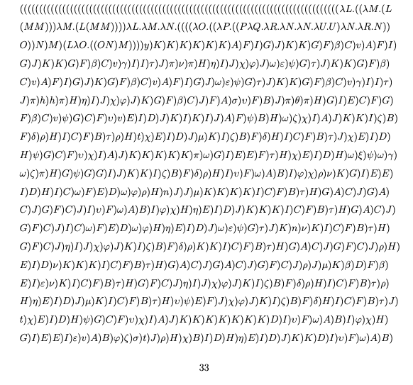
Here you can see lots of variables being applied to some lambda term shown on the top line, which actually represents string-concatenator.

This consecutive application causes a lot of consecutive (s. This makes page 32 entirely consist of (:

Language Features

The Memory Model for Persistent Bindings

let bindings are stored in the heap in the state and passed on as persistent bindings. Each let binding holds their own environment stack, and each environment stack points to its lexical parent environment stack. For example, the following LambdaLisp code:

;; LambdaLisp
(let ((x 10) (y 20))
  (setq x 5)
  (let ((f (lambda ...)) (a '(a b c)))
    (print x)
    ...)
  (let ((g (lambda ...)) (b '(a b c))
    (print b)
    ...)))

induces the following memory tree:

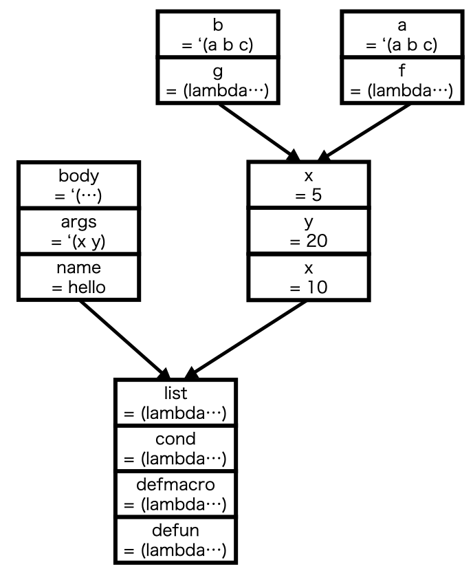
The node containing name = hello is not relevant now. The root node at the bottom contains bindings to basic functions initialized when running the prelude. This memory tree is expressed in the heap as:

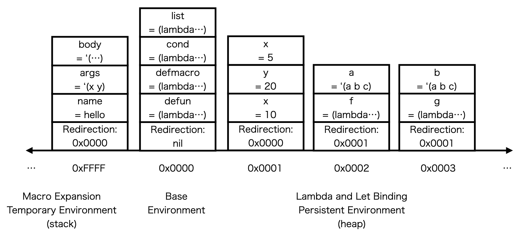
Here, the virtual RAM address space is shown as 16 bits for simplicity (the actual address space is 32 bits).

When a let binding occurs, the newest unallocated heap address is allocated my the malloc function, and the interpreter’s “current environment pointer” global variable contained in reg is rewritten to the newly allocated address. This also happens when a lambda is called, creating an environment binding the lambda arguments.

Each stack is initialized with a redirection pointer that points to its parent environment, shown at the bottom of the stack in the second figure. The bindings for each variable name is then pushed on top of the stack. On variable lookup, the lookup function first looks at the current environment’s topmost binding. If the target variable is not contained in the stack, the lookup reaches the redirection pointer at the bottom of the stack, where it will run the lookup again for the environment pointed by the redirection pointer. The lookup process ends when the redirection pointer is nil, where it concludes that the target variable is not bound to any value in the target environment. The use of the redirection pointer effectively models the environments’ tree structure.

For example, the x in the (print x) in the example code will invoke a lookup for x. The lookup function first looks at the binding stack at address 0x0002 and searches the stack until it reaches the redirection pointer to 0x0001. The lookup function then searches the binding stack at 0x0001, where it finds the newest binding of x which is x == 5. Since new bindings are pushed onto the stack, they get found before old bindings (here, x = 10) are reached.

Variable rewriting with setq is done by pushing assignments onto the stack. The (setq x 5) first searches for the variable x, finds it at environment 0x0001, then pushes x = 5 on top of y = 20 :: x = 10 on the environment 0x0001.

The address 0x0000 represents the base environment. It first starts out by being initialized by the function and macro definitions in the prelude. Variables stored in the base environment behave as global variables. This is where setq and defglobal behave differently. When (setq x ...) is called, setq first searches for x from the environment tree. If it finds x somewhere in the tree, it rewrites the found x at that environment. If it doesn’t find x, it defaults to pushing a new variable x to the current surrounding environment. This way, setq will only affect known variables or local variables. On the other hand, defglobal pushes the bindings to address 0x0000 no matter where it is called. This way, the address 0x0000 can behave as a global environment. The macro defun is defined using defglobal so that it always writes to the global environment. The macro defun-local is defined using setq so that it writes in the local environment, allowing for Python and JavaScript-style local function definitions:

;; LambdaLisp
(defun f (x y)
  (defun-local helper (z)
    (* z z))
  (print helper) ;; => @lambda
  (+ (helper x) (helper y)))

(print helper) ;; => (), since it is invisible from the global environment

Garbage Collection

Although there is no garbage collection for let and setq bindings, there is a minimal form of GC for macro expansion. During an evaluation of a macro, there occurs 2 Lisp form evaluations: one for constructing the expanded form, and another for evaluating the expanded form in the called environment. Once the macro has been expanded, we know for sure that the bindings it has used will not be used again. Therefore, macro bindings are allocated to the stack region which has negative addresses starting from 0xFFFF, shown on the left half of the memory tree diagram and the heap diagram. The stack region is freed once the macro expansion finishes. This mechanism also supports nested macros.

In the memory tree in the first figure in the previous section, the bindings for macros look the same as the bindings for lambdas, since at evaluation time they are treated the same. In the second figure, the environments for the macro bindings are shown on the left side of the RAM, since they are allocated in the stack region.

Although the same garbage-collection feature could be implemented for lambdas, it causes problems for lambdas that return closures. If lambda bindings are created in the stack region, the environment of the returned closure will point to the stack region, which will be freed right after the closure is returned. This causes a problem when the returned closure refers to a variable defined in the global environment (for example, to basic macros defined in the prelude such as cond), since the lookup function will eventually start looking at the stack region, which could be occupied by an old environment or some other lambda’s environment, causing the risk for bugs. This could be circumvented by carefully writing the code to not shadow global variables in let bindings, but that would severely restrict the coding style, so I chose to allocate new bindings for each lambda call. The growing memory can be freed by implementing a mark-and-sweep garbage collection function, which is currently not supported by LambdaLisp.

Macros

Macros are implemented as first-class objects in LambdaLisp. Both macros and lambdas are subtypes of the type lambda, each annotated with a subtype tag.

Macros are treated the same as lambdas, except for the following differences:

• The arguments are taken verbatim and are not evaluated before being bound to the argument variable names.
  • In lambdas, the arguments are evaluated before being bound.
• Two evaluations happen during a macro evaluation. The first evaluation evaluates the macro body to build the macro-expanded expression. The expanded expression is then evaluated in the environment which the macro was called.
  • In lambdas, only one evaluation (the latter one) happens.
• The first evaluation always has the base environment 0x00000000 set as its parent environment so that expansion always happens in the global environment, as explained in the previous section.
  • The second evaluation works the same as lambdas, where the environment where the macro/lambda was called is used for evaluation.
• The environment for the bound variables are stored in the stack region (negative addresses starting from 0xFFFFFFFF).
  • In lambdas, they are stored in the heap region (starting from 0x00000001).

An anonymous macro can be made with the macro keyword as (macro (...) ...), in the exact same syntax as lambdas. In the prelude, defmacro is defined as the following macro:

;; LambdaLisp
(defglobal defmacro (macro (name e &rest b)
  `(defglobal ,name (macro ,e (block ,name ,@b)))))

Object-Oriented Programming

In Let Over Lambda, it is mentioned that object-oriented programming can be implemented by using closures (Chapter 2). A primitive example is the counter example we’ve seen at the beginning:

(defun new-counter (init)
  ;; Return a closure.
  ;; Use the let over lambda technique for creating independent and persistent variables.
  (let ((i init))
    (lambda () (setq i (+ 1 i)))))

;; Instantiate counters
(setq counter1 (new-counter 0))
(setq counter2 (new-counter 10))

(print (counter1)) ;; => 1
(print (counter1)) ;; => 2
(print (counter2)) ;; => 11
(print (counter1)) ;; => 3
(print (counter2)) ;; => 12
(print (counter1)) ;; => 4
(print (counter1)) ;; => 5

LambdaLisp extends this concept and implements OOP as a predefined macro in the prelude. LambdaLisp supports the following Python-like object system with class inheritance:

(defclass Counter ()
  (i 0)

  (defmethod inc ()
    (setf (. self i) (+ 1 (. self i))))

  (defmethod dec ()
    (setf (. self i) (- (. self i) 1))))


(defclass Counter-add (Counter)
  (defmethod *init (i)
    (setf (. self i) i))

  (defmethod add (n)
    (setf (. self i) (+ (. self i) n))))


(defclass Counter-addsub (Counter-add)
  (defmethod *init (c)
    ((. (. self super) *init) c))

  (defmethod sub (n)
    (setf (. self i) (- (. self i) n))))


(defparameter counter1 (new Counter))
(defparameter counter2 (new Counter-add 100))
(defparameter counter3 (new Counter-addsub 10000))

((. counter1 inc))
((. counter2 add) 100)
((. counter3 sub) 10000)

(setf (. counter1 i) 5)
(setf (. counter2 i) 500)
(setf (. counter3 i) 50000)

Blocks

The notion of blocks in LambdaLisp is a feature borrowed from Common Lisp, close to for and break in C and Java. A block creates a code block that can be escaped by running (return [value]) or (return-from [name] [value]).

For example:

;; LambdaLisp
(block block-a
  (if some-condition
    (return-from block-a some-value))
  ...
  some-other-value)

Here, when some-condition is true, the return-from lets the control immediately break from block-a, setting the value of the block to some-value. If some-condition is false, the program proceeds until the end, and the value of the block becomes some-other-value, which is the same behavior as progn. Nested blocks are also possible, as shown in examples/block.cl.

defun is defined to wrap its content with an implicit block, you can write return-from statements with the function name:

;; LambdaLisp
(defun f (x)
  (if some-condition
    (return-from f some-value))
  (if some-condition2
    (return-from f some-value2)
  ...))

Here is the definition of defun in the prelude:

;; LambdaLisp
(defmacro defun (name e &rest b)
  `(defglobal ,name (lambda ,e (block ,name ,@b))))

In order to implement blocks, the interpreter keeps track of the name and the returning point of each block. This is done by preparing a global variable reg-block-cont in the register, used as a stack to push and pop name-returning-point pairs. Since LambdaCraft is written in continuation-passing style, the returning point is explicitly given as the callback function cont at any time in the eval function. Using this feature, when a block form appears, the interpreter first pushes the name and the current cont to the reg-block-cont global variable. The pushed cont is a continuation that expects the return value of the block to be applied as its argument. Whenever a (return-from [name] [value]) form is called, the interpreter searches the reg-block-cont stack for the specified [name]. Since the searched cont expects the return value of the block to be applied, the block escape control flow can be realized by applying [value] to cont, after popping the reg-block-cont stack.

Loops

A loop is a special form equivalent to while (true) in languages such as C, used to create infinite loops. A loop creates an implicit block with the name (), and can be exited by running (return) inside:

;; LambdaLisp
(defparameter i 0)
(loop
  (if (= i 10)
    (return))
  (print i)
  (setq i (+ i 1)))

Loops can also be exited by surrounding it with a block:

;; LambdaLisp
(defparameter i 0)
(block loop-block
  (loop
    (if (= i 10)
      (return-from loop-block))
    (print i)
    (setq i (+ i 1))))

Loops are implemented by passing a self-referenced continuation that runs the contents of loop again.

Error Invocation and Stack Traces

Some examples of situations when errors are invoked in LambdaLisp are:

• In read-expr:
  • When an unexpected ) is seen
• In eval:
  • When an unbound variable is being referenced
• In eval-apply (used when lambdas or macros are called):
  • When the value in the function cell does not belong to a subtype of lambda

When an error occurs during eval, read-expr or any function, the interpreter does the following:

• It immediately stops what it’s doing
• It shows an error message
• It shows the function call stack trace
• It returns to the REPL, awaiting the user’s input

Immediately stopping the current task and returning to the REPL is implemented very simply thanks to continuation-passing style. When an error is invoked, instead of calling the continuation (the callback), the repl function is called - this simple implementation allows error invocation.

Since invoking an error calls repl, and repl calls read-expr, eval and eval-apply, this makes the four functions read-expr, eval, eval-apply and repl be mutually recursive functions. How mutually recursive functions are implemented in LambdaLisp is described later in the next section.

The function call stack trace is printed by managing a call stack in one of the interpreter’s global variables. Every time a lambda or a macro is called, the interpreter pushes the expression that invoked the function call to the call stack. When the function call exits properly, the call stack is popped. When an error is invoked during a function call, the interpreter prints the contents of the call stack.

Other General Lambda Calculus Programming Techniques

Below are some other general lambda calclus programming techniques used in LambdaLisp.

Mutual Recursion

In LambdaCraft, recursive functions can be defined using defrec-lazy as follows:

;; LambdaCraft
(defrec-lazy fact (n)
  (if (<= n 0)
    1
    (* n (fact (- n 1)))))

defrec-lazy uses the Y combinator to implement anonymous recursion, a technique used to write self-referencing functions under the absence of a named function feature. Since LambdaLisp is based on macro expansion, when a self-referencing function is written using defun-lazy, the function body becomes infinitely expanded, causing the program to not compile. LambdaCraft shows an error message in this case. Using the Y combinator through defrec-lazy prevents this infinite expansion from happening.

Things get more complex in the case of what is called mutual recursion. In LambdaLisp, the functions read-expr, eval, eval-apply, and repl are mutually recursive, meaning that these functions call each other inside their definitions. Although using the normal Y combinator would still make the code compilable in this case, it makes the same function be inlined over and over again, severely expanding the total output lambda term size.

The redundant inlining problem can be solved if each function held a reference to each other. This can be done by implementing a multiple-function version of the Y combinator. The derivation of a fixed point combinator for mutual recursion is described very intuitively in Wessel Bruinsma’s blog post, A Short Note on The Y Combinator, in the section “Deriving the Y Combinator”. Below is a summary of the derivation process introduced in this post.

Suppose that we have two functions $f$ and $g$ that are mutually recursive. Since they reference each other in their definitions, $f$ and $g$ can be defined in terms of some function $h_f$ and $h_g$, which takes the definitions of $f$ and $g$ as its arguments:

$$\begin{aligned} f &:= h_f f g & (1)\\ g &:= h_g f g & (2)\\ \end{aligned}$$

$h_f$ and $h_g$ looks something like:

$$\begin{aligned} h_f &= \lambda f'. \lambda g'. \lambda x. k_f [f',g',x] \\ h_g &= \lambda f'. \lambda g'. \lambda x. k_g [f',g',x] \\ \end{aligned}$$

Where $k_* [f',g',x]$ is a term containing $f', g'$ and $x$.

Now suppose that $f$ and $g$ could be written using some unknown function $\hat f$ and $\hat g$ as:

$$\begin{aligned} f &:= \hat f \hat f \hat g \\ g &:= \hat g \hat f \hat g \end{aligned}$$

Plugging this into Equations (1) and (2),

$$\begin{aligned} \hat f \hat f \hat g &= h_f (\hat f \hat f \hat g) (\hat g \hat f \hat g ) \\ \hat g \hat f \hat g &= h_g (\hat f \hat f \hat g) (\hat g \hat f \hat g ) \\ \end{aligned}$$

Which can be abstracted as

$$\begin{aligned} \hat f \hat f \hat g &= (\lambda x. \lambda y. h_f (x x y) (y x y)) \hat f \hat g \\ \hat g \hat f \hat g &= (\lambda x. \lambda y. h_g (x x y) (y x y)) \hat f \hat g \\ \end{aligned}$$

Comparing both sides, we have

$$\begin{aligned} \hat f &= \lambda x. \lambda y. h_f (x x y) (y x y) \\ \hat g &= \lambda x. \lambda y. h_g (x x y) (y x y) \\ \end{aligned}$$

which are closed-form lambda expressions. Plugging this into our definitions $f := \hat f \hat f \hat g$ and $g := \hat g \hat f \hat g$, we get the mutually recursive definitions of $f$ and $g$.

A 4-function version of this mutual recursion setup is used in the init function in LambdaLisp to define repl, eval-apply, read-expr, and eval:

;; LambdaCraft
(let* read-expr-hat  (lambda (x y z w) (def-read-expr  (x x y z w) (y x y z w) (z x y z w) (w x y z w))))
(let* eval-hat       (lambda (x y z w) (def-eval       (x x y z w) (y x y z w) (z x y z w) (w x y z w))))
(let* eval-apply-hat (lambda (x y z w) (def-eval-apply (x x y z w) (y x y z w) (z x y z w) (w x y z w))))
(let* repl-hat       (lambda (x y z w) (def-repl       (x x y z w) (y x y z w) (z x y z w) (w x y z w))))
(let* repl       (repl-hat       read-expr-hat eval-hat eval-apply-hat repl-hat))
(let* eval-apply (eval-apply-hat read-expr-hat eval-hat eval-apply-hat repl-hat))
(let* read-expr  (read-expr-hat  read-expr-hat eval-hat eval-apply-hat repl-hat))
(let* eval       (eval-hat       read-expr-hat eval-hat eval-apply-hat repl-hat))

The functions *-hat and def-* each correspond to $\hat *$ and $h_*$ in the derivation. The final functions repl eval-apply read-expr eval are defined in terms of these auxiliary functions.

The functions def-* are defined in a separate location. def-eval, used to define eval, is defined as follows:

;; LambdaCraft
(defun-lazy def-eval (read-expr eval eval-apply repl expr state cont)
  ...)

def-eval is defined as a non-recursive function using defun-lazy, taking the four mutually dependent functions read-expr eval eval-apply repl as the first four arguments, followed by its “actual” arguments expr state cont. The first four arguments are occupied in the expression (def-read-expr (x x y z w) (y x y z w) (z x y z w) (w x y z w)) in the definition of read-expr-hat. By currying, this lets eval only take the 3 remaining unbound arguments, expr state cont.

Deriving ‘isnil’

isnil is one of the most important functions in cons-based lambda calculus programming, bearing the importance comparable to the atom special form in McCarthy’s original pure Lisp.

Consider the following function reverse that reverses a cons-based list:

;; LambdaCraft
(defrec-lazy reverse (l tail)
  (do
    (if-then-return (isnil l)
      tail)
    (<- (car-l cdr-l) (l))
    (reverse cdr-l (cons car-l tail))))

reverse is a recursive function that reverses a nil-terminated list made of cons cells. The base case used to end the recursion for reverse is when l is nil, decided by (isnil l).

Basically, any recursive function that takes a cons-based list must check if the incoming list is either a cons or a nil to write its base case. However, these data types have very different definitions:

$$\begin{aligned} {\rm cons} ~ A ~ B &:= \lambda f. (f ~ A ~ B) \\ {\rm nil} &:= \lambda x. \lambda y. y \end{aligned}$$

The function isnil must return ${\rm true} := \lambda x. \lambda y. x$ when its argument is ${\rm nil}$, and return ${\rm nil}$ when the argument is any ${\rm cons}$ cell. At first sight, it seems that this is impossible since there is no general way to check the equivalence of two given general lambda terms. Moreover, cons cells are a class of lambda terms that have the form $\lambda f. (f ~ A ~ B)$.

While checking the equivalence of general lambda terms is impossible due to the halting problem (c.f. here), it is possible for some cases of comparing between lambdas with predefined function signatures. This is also the case for isnil, where we can derive its concrete definition as follows.

First observe that a ${\rm cons}$ cell is a function that takes one callback function and applies to it the two values that it holds. On the other hand, ${\rm nil}$ is a function that takes two functions as its argument. This difference makes the following sequence of applications to turn out differently for ${\rm cons}$ and ${\rm nil}$:

$$\begin{aligned} ({\rm cons} ~ A ~ B) ~ (\lambda a. \lambda b. x) ~ c &= (\lambda f. (f ~ A ~ B)) ~ (\lambda a. \lambda b. x) ~ c \\ &= x ~ c \\ {\rm nil} ~ (\lambda a. \lambda b. x) ~ c &= (\lambda x. \lambda y. y) ~ (\lambda a. \lambda b. x) ~ c \\ &= c \\ \end{aligned}$$

Here, we applied $(\lambda a. \lambda b. x)$ and $c$ to $({\rm cons} ~ A ~ B)$ and ${\rm nil}$, where $x$ and $c$ are free variables. Notice that the abstractions in $(\lambda a. \lambda b. x)$ are used to ignore the values contained in the ${\rm cons}$ cell.

These sequences of applications can directly be used to define ${\rm isnil}$. To implement ${\rm isnil}$, we want the latter expression to evaluate to ${\rm true}$. This can be done by setting $c := {\rm true}$.

It then remains to find an $x$ where $(x ~ c) = (x ~ {\rm true}) := {\rm nil}$. From here we immediately get $x := \lambda w. {\rm nil}$.

Therefore, ${\rm isnil}$ can be written by abstracting this process:

$$\begin{aligned} {\rm isnil} &= \lambda z. (z ~ (\lambda a. \lambda b. \lambda w. {\rm nil}) ~ {\rm true}) \\ &= \lambda z. (z ~ (\lambda a. \lambda b. \lambda w. \lambda x. \lambda y. y) ~ (\lambda x. \lambda y. x)) \\ \end{aligned}$$

which can be used as

$$\begin{aligned} {\rm isnil} ~ ({\rm cons} ~ A ~ B) &= {\rm nil} \\ {\rm isnil} ~ {\rm nil} &= {\rm true} \end{aligned}$$

The pattern $\lambda a. \lambda b. \lambda w. \lambda x. \lambda y. y$ is noticable in many places in lambdalisp.pdf, since isnil is used a lot of times in LambdaLisp.

LambdaCraft’s ‘do’ Macro

The heavy use of CPS in LambdaLisp is supported by LambdaCraft’s do macro. Writing raw code in CPS causes a heavily nested code, since CPS is based on callbacks. The do macro makes such nested code to be written as flat code, in a syntax close to Haskell’s do notation for monads.

Here is the do notation in Haskell:

do
  (y, z) <- f x
  w <- g y z
  return w

A similar code can be written in LambdaCraft as:

(do
  (<- (y z) (f x))
  (<- (w) (g y z))
  w)

which is macro-expanded to:

(f x
  (lambda (y z)
    (g y z
      (lambda (w)
        w))))

where f, g is defined in CPS:

(defun-lazy f (x cont) ...)
(defun-lazy g (y z cont) ...)

Here, the cont represents the callback function, which is directly written as the inner lambdas.

Print Debugging

The return type of eval is string, and not expr. This is because expr is “returned” with CPS, by applying it to the provided callback:

;; LambdaCraft
(eval expr state
  (lambda (eval-result state)
    [do something with eval-result and state]))

This is written using do as:

(do
  (<- (eval-result state) (eval expr state)
  [do something with eval-result and state]))

The nice part about the do macro and having eval return strings is that it makes print debugging very intuitive. Since LambdaLisp is written in CPS, an arbitrary point in the eval function eventually becomes the head of the current evaluation. Therefore, at any point in the program, you can write

;; LambdaCraft
(eval expr state
  (lambda (eval-result state)
    (cons "a" (cons "b" (cons "c" [do something with eval-result and state])))))

which will make the entire expression eventually evaluate to

;; LambdaCraft
;; The outermost expression
(cons "a" (cons "b" (cons "c" ...)))

which will print “abc” in the console.

The previous code can be written in imperative style using do as

;; LambdaCraft
(do
  (<- (eval-result state) (expr state))
  (cons "a")
  (cons "b")
  (cons "c")
  [do something with eval-result and state])

which is virtually identical to writing (print "a") in an imperative language. Note that the default behavior of do is to nest the successive argument at the end of the list, starting from the last argument, and <- is a specially handled case by do.

(cons "a") can be replaced with a string printing function that accepts a continuation, such as:

;; LambdaCraft
(defun-lazy show-message (message state cont)
  (do
    (print-string message)
    (cons "\\n")
    (cont state)))

which will print message, print a newline, and proceed with (cont state).

This design was very helpful during debugging, since it let you track the execution flow using print debugging. This design and technique can be used in other general lambda-calculus based programs as well.

Type Checking with Macro Call Signatures

Another large-scale programming technique is using macro signatures as a type-checking functionality.

Since all lambdas defined by def-lazy, defun-lazy or defrec-lazy are curried in LambdaCraft, there is no simple way to tell how many arguments a lambda that is being called takes. This is different for LambdaCraft macros defined by defmacro-lazy, since LambdaCraft macros are implemented as Common Lisp functions that run on the Common Lisp environment to expand the macro at compile time. Therefore, when a LambdaCraft macro is called with excessive or insufficient number of arguments, it causes a Common Lisp error at compile time. This works as a strong macro signature type-checker which significantly helps the debugging process of LambdaCraft, letting you know when a LambdaCraft macro is called with insufficient arguments. This effectively works as a simple type checker for macro call signatures. The Common Lisp call stack even tells you which line got the macro call wrong which helps debugging as well. It is therefore convenient to use as much macros as possible when writing programs in LambdaCraft.

Writing in terms of macros help reduce the code size as well, since using macros can be seen as running compile-time beta reductions beforehand of the runtime. For example, while cons can be written as a function (defun-lazy cons (x y) (lambda (f) (f x y))), it can also be written as a macro (defmacro-lazy cons (x y) `(lambda (f) ,x ,y)), which is the beta-reduced form of the function-based definition. Either code will evaluate the same results by writing (cons p q), except the function-based one requires an extra beta-reduction step at runtime, affecting the performance.

Appendix

JavaScript Examples of Continuation-Passing Style Code

CPS causes the largest impact when extracting the values of a cons cell. This is illustrated in the JavaScript code below that runs on a browser’s JavaScript console.

In direct style, destructing a value of a cons tuple is written as:

// Runs on the browser's JavaScript console
function car (x) {
    return x(function (a, b) { return a; });
}
function cdr (x) {
    return x(function (a, b) { return b; });
}

function cons (a, b) {
    return function (f) {
        return f(a,b);
    };
}
function t (a, b) {
    return a;
}
function nil (a, b) {
    return b;
}

(function(x) {
    return (function (y) {
        return (function (z) {
            return z(z, z);
        })(car(y));
    })(cdr(x));
})(cons(t, cons(nil, t)))

The last expression in this code first binds (cons t (cons nil t)) to x, and calculates (car (cdr x)). Running this on the browser’s console should return the function nil.

The car and cdr correspond to the following lambda terms that accept a data and return the data in the desired position:

$$\begin{aligned} {\rm car} &= \lambda x. \lambda y. x \\ {\rm cdr} &= \lambda x. \lambda y. y \\ \end{aligned}$$

On the other hand, in continuation-passing style, the same code is written as:

// Runs on the browser's JavaScript console
function cons (a, b) {
    return function (f) {
        return f(a,b);
    };
}
function t (a, b) {
    return a;
}
function nil (a, b) {
    return b;
}

cons(t, cons(nil, t))(            // cons returns a function that accepts a callback function. We pass a callback to it
    function (tmp1, y){           // This function works as cdr; It takes the second value (and discards the first)
        return y(                 // y == cons(nil, t) now. Inside, we write what we want to do with the y we receive via the callback. Here we pass another callback to the return value of the inner cons.
            function (z, tmp2) {  // This function works as car; It takes the first value (and discards the second)
                return z(z, z);   // z == nil now. nil selects the second value among its arguments, which here evaluates to nil.
            }
        );
    }
)

Here, values are extracted without using car or cdr at all. It instead uses the fact that a cons cell is actually a function that accepts a callback function that applies both of its contents to the provided callback.

This significantly improves performance when reading the stdin, which is a list made from cons cells:

;; LambdaCraft
(stdin
  (lambda (c cdr-stdin)
    (if (=-bit c "(")
      ...)))

The Binary Lambda Calculus Notation

The interpreters Blc, tromp, and uni runs programs writen in binary lambda calculus (BLC - also see here). The difference between binary lambda calculus and ordinary lambda calculus is in the notation, i.e. how lambda terms are written, and everything else including the rules of beta reduction are the same. BLC’s notation is based on De Bruijn notation, where variable names such as $x, y$ and $z$ are eliminated, and are instead replaced by an integer describing the relative nesting depth distances viewed from the variable’s surrounding scope.

The De Bruijn notation works as follows. Consider for example the term $\lambda x. \lambda y. \lambda z. y$. Here, from the eyes of the term $y$, the originating lambda of the variable $y$ is reached by hopping 1 abstraction $\lambda z$, so the De Bruijn index for the term $y$ is 1. We can therefore rewrite as

$$\lambda x. \lambda y. \lambda z. y = \lambda x. \lambda y. \lambda z. 1$$

and still recover its meaning. Similarly, The index for $x$ in $\lambda x. \lambda y. \lambda z. x$ would be 2, and for $z$ in $\lambda x. \lambda y. \lambda z. z$ would be 0 since no hops are required. This works for a more complicated setting, for example in $\lambda x. (x \lambda y. \lambda z.((x z) y))$ the index for $y$ is 1. $x$ occurs twice in this term, and each are encoded differently in this case. The innermost $x$ has index 2 since 2 hops is required past $\lambda z$ and $\lambda y$, but the outer $x$’s index is 0 since no hops are required to reach $\lambda x$ in the eyes of the outermost $x$. We can then write

$$\lambda x. (x \lambda y. \lambda z.((x z) y)) = \lambda x. (0 \lambda y. \lambda z.((2 0) 1))$$

and we can still deduce which variable each integer corresponds to.

We then notice that when written in De Bruijn indices, the variable names in the lambda declaration becomes entirely redundant. The expression can thus be rewritten as

$$\begin{aligned} \lambda x. (x \lambda y. \lambda z.((x z) y)) &= \lambda x. (0 \lambda y. \lambda z.((2 0) 1)) \\ &= \lambda (0 \lambda \lambda ((2 0) 1)) \end{aligned}$$

and it would still hold the same meaning.

We can simplify the notation more by writing function application $(A B)$ as ${\rm apply}~A~B$. Doing this we get:

$$\begin{aligned} \lambda x. (x \lambda y. \lambda z.((x z) y)) &= \lambda (0 \lambda \lambda ((2 0) 1)) \\ &= \lambda ~ {\rm apply} ~ 0 ~ \lambda \lambda ~{\rm apply} ~ {\rm apply} ~ 2 ~ 0 ~ 1 \end{aligned}$$

By assuming that ${\rm apply}$ always takes exactly 2 parameters, we can eliminate the need for writing parentheses to express ${\rm apply}$.

Binary lambda calculus then encodes this sequence as follows:

$$\begin{aligned} \lambda &= 00 \\ {\rm apply} &= 01 \\ i &= 1^{i+1}0 \\ \end{aligned}$$

We thus have

$$\begin{aligned} \lambda x. (x \lambda y. \lambda z.((x z) y)) &= \lambda ~ {\rm apply} ~ 0 ~ \lambda \lambda ~{\rm apply} ~ {\rm apply} ~ 2 ~ 0 ~ 1 \\ &= 00~01~10~00~00~01~01~1110~10~110 \end{aligned}$$

which completes the definition of the binary lambda calculus notation.

The Blc interpreter (and the Universal Lambda interpreter) accepts this bitstream and parses it to a lambda term, which then applies beta reduction to execute the program.

Some more examples are

$$\begin{aligned} \lambda x. x &= \lambda 0 &= 00~10 \\ \lambda x. \lambda y. x &= \lambda \lambda 1 &= 00~00~110 \\ (\lambda x. x) (\lambda x. x) &= {\rm apply}~ \lambda 0 ~ \lambda 0 &= 01~00~10~00~10 \end{aligned}$$

The elegance of this notation is that it is a prefix code, so no delimiting characters are required - the spaces between the $0$ and $1$ can be removed in practice. Moreover, for any valid proram $P$, there exists no valid program $PQ$ that starts with $P$ followed with a nonempty $Q$.

Due to the prefix code property, the interpreter can distinguish the boundary between the program and the stdin even if they are provided as concatenated byte streams. For example, when running lambdalisp.blc, we run:

cat lambdalisp.blc | ./asc2bin > lambdalisp.blc.bin
cat lambdalisp.blc.bin [filepath] | ./Blc

Normally, it is difficult or impossible to deduce the boundary between the binary lambdalisp.blc.bin and [filepath] since they are cated together, but it is easily possible in BLC since all valid programs are prefix codes.

About the Logo

• The rounded edges of the cube represent Lisp’s parentheses syntax.
• Alan Kay described Lisp in the quote, “Lisp isn’t a language, it’s a building material.” The cube is a depiction of a block, which represents the building blocks of software.

Credits

LambdaLisp was written by Hikaru Ikuta. The lambda calculus term compiler LambdaCraft was written by Hikaru Ikuta, inspired by Ben Rudiak-Gould’s Scheme program Lazier, a compiler from lambda terms written in Scheme to Lazy K. The LambdaLisp logo was designed by Hikaru Ikuta. The 521-byte lambda calculus interpreter SectorLambda was written by Justine Tunney. The IOCCC 2012 “Most functional” interpreter was written by John Tromp. The Universal Lambda interpreter clamb and Lazy K interpreter lazyk was written by Kunihiko Sakamoto.