Building a Neural Network in Pure Lisp Without Built-In Numbers Using Only Atoms and Lists

At the dawn of Lisp after its birth in 1958, Lisp was used as a language for creating advanced artificial intelligence. This project makes that a reality once again by implementing a neural network for pattern recognition written in pure lisp without built-in integers or floating-point numbers, that runs on the IBM PC model 5150.

Building Neural Networks only using Symbolic Manipulation

SectorLISP is an amazing project where a fully functional Lisp interpreter is fit into the 512 bytes of the boot sector of a floppy disk. Since it works as a boot sector program, the binary can be written to a disk to be used as a boot drive, where the computer presents an interface for writing and evaluating Lisp programs, all running in the booting phase of bare metal on the 436-byte program. I have written another blog post on SectorLISP about extending SectorLISP to implement BASIC REPLs and games.

SectorLISP is implemented as a pure Lisp. In pure Lisp, there are no built-in types for integers or floating-point numbers, and only supports atoms and lists as available data structures. Surprisingly, even with the lack of numbers, such a Lisp is Turing-complete, meaning that it is basically capable of any calculation that can be done on modern computers.

In this project, we implement a neural network that runs on SectorLISP. Since there are no features of built-in numbers, we have to reinvent the notion of numbers from scratch only by using symbolic manipulation. We first start off by constructing a fixed-point number calculation system based solely on list manipulations, and finally, implement matrix multiplication and activation functions using this fixed-point number system.

Since SectorLISP runs on the IBM PC model 5150, this implementation allows neural networks to run on the booting phase of vintage PCs.

Running the Neural Network on Your Computer

The source code for the SectorLISP neural network, as well as the training and testing scripts used to obtain the model parameters, are available at my GitHub repository:

https://github.com/woodrush/sectorlisp-nn

Here I will describe the instructions for running the SectorLISP program to calculate predictions for custom digit images in detail. The instructions for training and evaluating the neural network to obtain the model parameters used for this network is available at the repository.

The available emulators are QEMU and the i8086 emulator Blinkenlights. I will also describe how to run SectorLISP on physical hardware, except for this method you must type the entire Lisp program by hand into the computer. In the emulators, you can either automatically load the code or paste it into the console.

Running on QEMU

If you have QEMU installed, running the Lisp neural network on QEMU can be done by running the following make prodedure:

git clone https://github.com/woodrush/sectorlisp
git checkout nn
git submodule update --init --recursive
cd test
make nn

This will start QEMU with SectorLISP loaded as the boot sector program, and will automatically type the Lisp program into the emulator’s console.

Due to the way the test script handles the text stream between the host PC and QEMU, it first takes 10 minutes to type the entire Lisp source code to the emulator’s console. After waiting for 10 minutes, the actual inference time only takes about 4 seconds, where the program will show a message on the screen indicating the predicted digit. The running time was measured using a 2.8 GHz Intel i7 CPU.

To input a custom 3x5 digit image, edit the following expression at the end of the program, ./sectorlisp-nn/nn.lisp, inside the sectorlisp-nn submodule:

 (QUOTE
   ;; input
 )
 (QUOTE (* * *
         * . .
         * * *
         . . *
         * * *))

Running on Blinkenlights

Here are the instructions on running the network on the i8086 emulator Blinkenlights.

First, git clone the SectorLISP repository and make SectorLISP’s binary, sectorlisp.bin:

git clone https://github.com/jart/sectorlisp
cd sectorlisp
make

This will generate sectorlisp.bin under ./sectorlisp.

By building a fork of SectorLISP that supports I/O, an additional output with some messages indicating the input and the output will become printed. In this case, git checkout to the io branch by running git checkout io before running make. Since the source code for this project is backwards comptible with the main SectorLISP branch, the same code can be run on both versions.

Update (2022/4/6): The fork mentioned here was merged into the original SectorLISP repository. The features mentioned here can now be used without using the fork, and by using the original SectorLISP repository.

To run SectorLISP on Blinkenlights, first follow the instructions on its download page and get the latest version:

curl https://justine.lol/blinkenlights/blinkenlights-latest.com >blinkenlights.com
chmod +x blinkenlights.com

You can then run SectorLISP by running:

./blinkenlights.com -rt sectorlisp.bin

In some cases in Ubuntu, there might be a graphics-related error showing and the emulator may not start. In that case, run the following command first available on the download page:

sudo sh -c "echo ':APE:M::MZqFpD::/bin/sh:' >/proc/sys/fs/binfmt_misc/register"

Running this command should allow you to run Blinkenlights on your terminal. Instructions for running Blinkenlights on other operating systems is described in the Blinkenlights download page.

After starting Blinkenlights, expand the size of your terminal large enough so that the TELETYPEWRITER region shows up at the center of the screen. This region is the console used for input and output. Then, press c to run the emulator in continuous mode. The cursor in the TELETYPEWRITER region should move one line down. You can then start typing in text or paste a long code from your terminal into Blinkenlight’s console to run your Lisp program.

To run the neural network program, copy the contents of nn.lisp from the repository to your clipboard, and paste it inside the terminal into Blinkenlight’s console. After waiting for about 2 minutes, the result will be shown on the console. Note that it is important to copy the newline at the end of the program, which will trigger the turbo mode on Blinkenlights which makes it run significantly faster. In this case, the screen will initially show nothing after you paste the code, but you can confirm that it is running by checking the CPU usage of your computer. If the code shows up right away after pasting with the cursor right next to the final parentheses of the code, you may have not included the newline, which takes significantly more time since it does not run in turbo mode.

On Blinkenlights, it took 2 minutes from pasting the code to obtaining the final inference results. The running time was measured using a 2.8 GHz Intel i7 CPU.

To input a custom 3x5 digit image, edit the following expression at the end of the program:

 (QUOTE
   ;; input
 )
 (QUOTE (* * *
         * . .
         * * *
         . . *
         * * *))

Running on Physical Hardware

You can also run SectorLISP on an actual physical machine if you have a PC with an Intel CPU that boots with a BIOS, and a drive such as a USB drive or a floppy disk that can be used as a boot drive. Note that when running the neural network program this way, you must type the entire program by hand into the console.

First, mount your drive to the PC you’ve built sectorlisp.bin on, and check:

lsblk -o KNAME,TYPE,SIZE,MODEL

Among the list of the hardware, check for the device name for your drive you want to write SectorLISP onto. After making sure of the device name, run the following command, replacing [devicename] with your device name. [devicename] should be values such as sda or sdb, depending on your setup.

Caution: The following command used for writing to the drive will overwrite anything that exists in the target drive’s boot sector, so it’s important to make sure which drive you’re writing into. If the command or the device name is wrong, it may overwrite the entire content of your drive or other drives mounted in your PC, probably causing your computer to be unbootable (or change your PC to a SectorLISP machine that always boots SectorLISP, which is cool, but is hard to recover from). Please perform these steps with extra care, and at your own risk.

sudo dd if=sectorlisp.bin of=/dev/[devicename] bs=512 count=1

After you have written your boot drive, insert the drive to the PC you want to boot it from. You may have to change the boot priority settings from the BIOS to make sure the PC boots from the target drive. When the drive boots successfully, you should see a cursor blinking in a blank screen, which indicates that you’re ready to type your Lisp code into bare metal.

We will now discuss the implementation details of this project.

Training the Neural Network

We first start off by training a neural network on a modern computer using TensorFlow to get its model parameters. The parameters are then converted to 18-bit fixed-point numbers when loading to the SectorLISP program.

The Dataset

Training Dataset

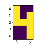
Test Dataset

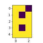
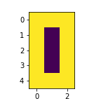
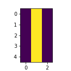
The entire dataset for training and testing this neural network is shown above. The input images are 3x5-sized binary monochrome images, which are converted to fixed-point vectors when being provided to the network.

The dataset, as well as the fully connected neural network model, were inspired by a blog post (in Japanese) about pattern recognition using neural networks, written by Koichiro Mori (aidiary).

The upper half is the training dataset that is used to train the neural network. The bottom half is the testing dataset, which is not shown at all to the network at training time, and will be shown for the first time when evaluating the neural network’s performance, to check if the digits for these newly shown images are predicted correctly.

In the final Lisp program, the input image is provided as follows:

(QUOTE
  ;; input
)
(QUOTE (* * *
        * . .
        * * *
        . . *
        * * *))

The Model

The model for our neural network is very simple. It is a two-layered fully connected network with a ReLU activation function:

In TensorFlow, it is written like this:

model = tf.keras.models.Sequential([
  tf.keras.layers.Flatten(input_shape=(5, 3)),
  tf.keras.layers.Dense(10, activation="relu"),
  tf.keras.layers.Dropout(0.2),
  tf.keras.layers.Dense(10),
])

The model and its implementation were referenced from the TensorFlow 2 quickstart for beginners entry from the TensorFlow documentation. As mentioned before, the fully-connected model was also inspired by a blog post (in Japanese) written by Koichiro Mori (aidiary).

This model takes a 3x5 image and outputs a 1x10 vector, where each element represents the log-confidence of each digit from 0 to 9. The final prediction result of the neural network is defined by observing the index that has the largest value in the output 1x10 vector.

Each fully connected neural network contains two trainable tensors A and B, which are the coefficient matrix and the bias vectors, respectively. This network thus consists of 4 model parameter tensors, A_1, B_1, A_2, and B_2, each of size 15x10, 10x1, 10x10, and 10x1, respectively.

The Dropout function is included for inducing generalization and is only activated at training time.

We use the categorical cross-entropy loss and the Adam optimizer for training:

model.compile(optimizer="adam",
             loss=tf.keras.losses.SparseCategoricalCrossentropy(from_logits=True),
             metrics=["accuracy"])

The model is then trained for 1000 epochs:

model.fit(data_x, data_y_category, epochs=1000, verbose=0)

After training, the model parameters are saved:

model.save("params.h5")

The model parameters A_1, B_1, A_2, and B_2 are contained in this file. Since each model parameter has the sizes 15x10, 10x1, 10x10, and 10x1, the total number of fixed-point numbers is 1620. Since we are using 18 bits for each fixed-point number, the total number of bits for the model parameters of the entire neural network is 29160 bits.

Note that although fixed-point numbers are used in the final Lisp implementation, the training process uses 64-bit floating-point numbers. Since the number of layers and the matrix sizes were both small enough for truncating the precision, we were able to directly convert the trained floating-point model parameter values to fixed-point numbers when loading them into the Lisp implementation.

The training time for the neural network in TensorFlow was 6.5 seconds on a 6GB GTX 1060 GPU.

Testing for Noise Resistance

The training accuracy was 100%, meaning that all of the 15 images in the training dataset are correctly predicted to the true digit.

The testing accuracy was 85%, meaning that 17 out of 20 newly seen images that were not shown at all during training were predicted correctly.

Here is the confusion matrix for the test dataset:

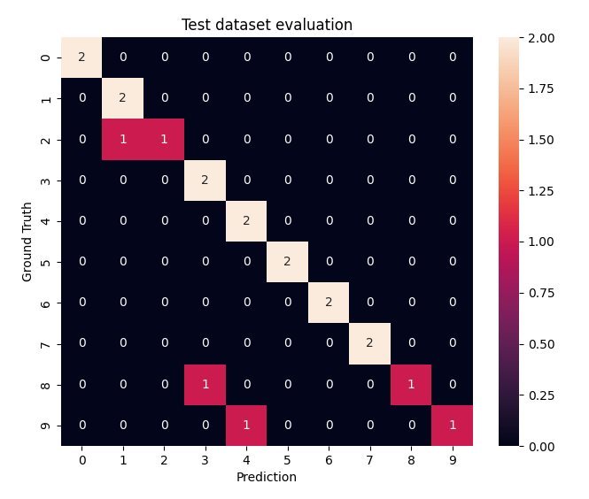
In the case for a 100% accuracy performance, the matrix becomes completely diagonal, meaning that the prediction results always match the ground truth labels. The three off-diagonal elements indicate the 3 prediction errors that occurred at test time.

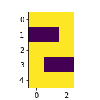
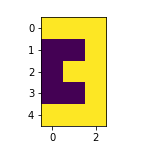
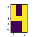
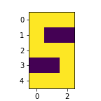
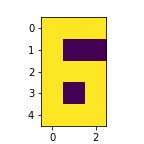
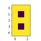
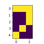
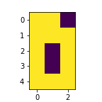
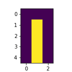
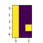
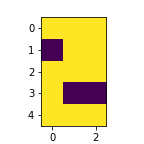
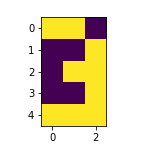
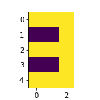
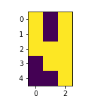
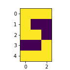
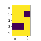
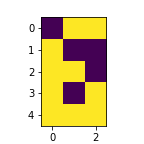
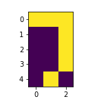
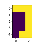
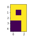
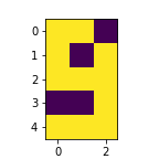
Here are the 3 images that were not predicted correctly:

Test Dataset Image	Prediction
	1
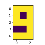
	3
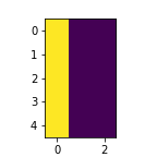
	4

Since all of the other images were predicted correctly, this means that the neural network was able to correctly predict 85% of the unknown data that was never shown at training time. This capability of flexible generalization for newly encountered images is a core feature of neural networks.

Implementing Neural Networks in Pure Lisp

“Lisp has jokingly been called “the most intelligent way to misuse a computer”. I think that description is a great compliment because it transmits the full flavor of liberation: it has assisted a number of our most gifted fellow humans in thinking previously impossible thoughts.” – Edsger W. Dijkstra

Now that we have obtained the model parameters for our neural network, it’s time to build it into pure Lisp.

As explained in the SectorLISP blog post, SectorLISP does not have a built-in feature for integers or floating-point numbers. The only data structures that SectorLISP has are lists and atoms, so we must implement a system for calculating fractional numbers only by manipulating lists of atoms. Our goal is to implement matrix multiplication in fixed-point numbers.

The fixed-point number system used in this project is also available as a SectorLISP library at my numsectorlisp GitHub repo.

The Number Representations

The number system for this project will be 18-bit fixed-point numbers, with 13 bits for the fractional part, 4 bits for the integer part, and 1 bit for the sign.

Here are some examples of numbers expressed in this fixed-point system:

(QUOTE (0  0 0 0 0  0 0 0 0  0 0 0 0    0 0 0 0 0)) ;; Zero
(QUOTE (0  0 0 0 0  0 0 0 0  0 0 0 0    1 0 0 0 0)) ;; One
(QUOTE (0  0 0 0 0  0 0 0 0  0 0 0 1    0 0 0 0 0)) ;; 0.5
(QUOTE (0  0 0 0 0  0 0 0 0  0 0 1 0    0 0 0 0 0)) ;; 0.25
(QUOTE (0  0 0 0 0  0 0 0 0  0 0 0 0    1 1 1 1 1)) ;; -1
(QUOTE (0  0 0 0 0  0 0 0 0  0 0 0 1    1 1 1 1 1)) ;; -0.5
(QUOTE (0  0 0 0 0  0 0 0 0  0 0 1 1    1 1 1 1 1)) ;; -0.25
(QUOTE (1  1 1 1 1  1 1 1 1  1 1 1 1    1 1 1 1 1)) ;; Negative epsilon (-2^13)
;;     |----------------------------|  |------||-|
;;            Fractional part       Integer part \Sign bit

Half Adder

We first start by making a half adder, which computes single-digit binary addition. A half adder takes the binary single-digit variables A and B and outputs a pair of variables S and C, each representing the sum and the carry flag. The carry C occurs when both input numbers are 1 needing a carry digit for addition. Therefore, it can be written as:

(QUOTE
  ;; addhalf : Half adder
)
(QUOTE (LAMBDA (X Y)
  (COND
    ((EQ X (QUOTE 1))
     (COND
       ((EQ Y (QUOTE 1)) (CONS (QUOTE 0) (QUOTE 1)))
       ((QUOTE T) (CONS (QUOTE 1) (QUOTE 0)))))
    ((QUOTE T)
     (CONS Y (QUOTE 0))))))

Full Adder

Next we make a full adder. A full adder also computes single-digit binary addition, except it takes 3 variables including the carry digit, A, B, and C, and outputs the pair S and C for the sum and the carry flag. Including C will help to recursively compute multiple-digit addition in the next section. This can be written as:

(QUOTE
  ;; addfull : Full adder
)
(QUOTE (LAMBDA (X Y C)
  ((LAMBDA (HA1)
     ((LAMBDA (HA2)
        (CONS (CAR HA2)
              (COND
                ((EQ (QUOTE 1) (CDR HA1)) (QUOTE 1))
                ((QUOTE T) (CDR HA2)))))
      (addhalf C (CAR HA1))))
   (addhalf X Y))))

Unsigned Integer Addition

Now that we have constructed a full adder, we can recursively connect these full adders to construct a multiple-binary-digit adder. We first start off by constructing an adder for unsigned integers.

Addition is done by first adding the least significant bits, computing the sum and the carry, and then adding the next significant bits as well as the carry flag if it exists. Since the full adder does just this for each digit, we can recursively connect full adders together to make a multiple-digit adder:

(QUOTE
  ;; uaddnofc : Unsigned N-bit add with carry
  ;;            The output binary is in reverse order (the msb is at the end)
  ;;            The same applies to the entire system
)
(QUOTE (LAMBDA (X Y C)
  (COND
    ((EQ NIL X) Y)
    ((EQ NIL Y) X)
    ((QUOTE T)
     ((LAMBDA (XYC)
        (CONS (CAR XYC) (uaddnofc (CDR X) (CDR Y) (CDR XYC))))
      (addfull (CAR X) (CAR Y) C))))))

Here, X and Y are multiple-digit numbers such as (QUOTE (0 0 0 0 0 0 0 0 0 0 0 0 0 1 0 0 0 0)) ;; One, and C is a single-digit carry flag.

This is where the reverse-ordered binary list format becomes useful. Since addition is started by adding the least significant bits first, we can immediately extract this bit just by applying (CAR X) to the numbers.

The u stands for unsigned, addn means the addition of N (arbitrary) digits, of means that overflow is prevented, c means that there is a carry flag as an argument. Since overflow is prevented, this means that the resulting sum may become one digit longer than the original inputs X and Y, instead of overflowing to zero. This is compensated later in other functions.

Finally, to add two unsigned integers X and Y, we wrap uaddnofc with the carry flag initially set to 0, for unsigned integer addition:

(QUOTE
  ;; uaddnof : Unsigned N-bit add
)
(QUOTE (LAMBDA (X Y)
  (uaddnofc X Y (QUOTE 0))))

Unsigned Integer Multiplication

Multiplication can be done similarly with addition, except we add multiple digits instead of one in each step. In multiplication, we recursively shift X one by one bit and add them up, when the corresponding digit in Y is 1. When the digit in Y is 0, we add nothing. Shifting X to the right has the effect of multiplying the number by 2. Note that the shifting effect is reversed since the bit order is reversed.

Following this design, unsigned integer multiplication is implemented as follows:

(QUOTE
  ;; umultnof : Unsigned N-bit mult
)
(QUOTE (LAMBDA (X Y)
  (COND
    ((EQ NIL Y) u0)
    ((QUOTE T)
     (uaddnof (COND
                ((EQ (QUOTE 0) (CAR Y)) u0)
                ((QUOTE T) X))
              (umultnof (CONS (QUOTE 0) X) (CDR Y)))))))

Unsigned Fixed-Point Addition

Now we are ready to start thinking about fixed-point numbers. In fact, we have already implemented unsigned fixed-point addition at this point. This is because of the most significant feature for fixed-point numbers, where addition and subtraction can be implemented exactly the same as signed integers.

This is because fixed-point numbers can be thought of as signed integers with a fixed exponent bias 2^N. Since the fraction part for our system is 13, the exponent bias is 2^(-13) for our system. Therefore, for two numbers A_fix and B_fix, we represent these numbers using an underlying integer A and B, as A_fix == A * 2^(-13), B_fix == B * 2^(-13).

Now, when calculating A_fix + B_fix, the exponent 2^(-13) can be factored out, leaving (A+B)*2^(-13). Therefore, we can directly use unsigned integer addition for unsigned fixed-point addition.

Unsigned Fixed-Point Multiplication

Multiplication is similar except that the exponent bias changes. For A_fix * B_fix in the previous example, the result becomes (A*B)*2^(-26), with a smaller exponent bias factor. Here, we have a gigantic number A*B compensated with the small exponent bias factor 2^(-26). Therefore, to adjust the exponent bias factor, we can divide A*B by 2^13, and drop the exponent bias factor to 2^(-13). In this case, dividing by 2^13 means to drop 13 of the least significant bits and to keep the rest.

In the case where the output number still has a bit length longer than A and B, this means that the result overflowed and cannot be captured by the number of bits in our system. This is the difference between floating-point numbers. For floating-point numbers, the most significant bit can always be preserved by moving around the decimal point. In fixed-point numbers, on the other hand, large numbers must have their significant bits discarded since the decimal point is fixed. Therefore, it is a little odd to drop the significant bits, but this implementation yields the correct results.

Following this design, we can implement unsigned fixed-point multiplication as follows:

(QUOTE
  ;; ufixmult : Unsigned fixed-point multiplication
)
(QUOTE (LAMBDA (X Y)
  (take u0 (+ u0 (drop fracbitsize (umultnof X Y))))))
(QUOTE

u0 indicates the unsigned integer zero, and fracbitsize is a list of length 13 indicating the fraction part’s bit size.

u0 is added after dropping bits from the multiplication result, since the bit length may be shorter than our system after dropping the bits.

take and drop are defined as follows:

(QUOTE
  ;; take : Take a list of (len L) atoms from X
)
(QUOTE (LAMBDA (L X)
  (COND
    ((EQ NIL L) NIL)
    ((QUOTE T) (CONS (CAR X) (take (CDR L) (CDR X)))))))
(QUOTE
  ;; drop : Drop the first (len L) atoms from X
)
(QUOTE (LAMBDA (L X)
  (COND
    ((EQ NIL X) NIL)
    ((EQ NIL L) X)
    ((QUOTE T) (drop (CDR L) (CDR X))))))

Negation

Now we will start taking the signs of the numbers into account.

In our fixed-point number system, negative numbers are expressed by taking the two’s complement of a number. Negation using two’s complement is best understood as taking the additive inverse of the number in mod (2^13)-1. This yields a very simple implementation for negation:

(QUOTE
  ;; negate : Two's complement of int
)
(QUOTE (LAMBDA (N)
  (take u0 (umultnof N umax))))

Here, umax is a number filled with 1, (QUOTE (1 1 1 1 1 1 1 1 1 1 1 1 1 1 1 1 1 1)). When added by the smallest positive number (QUOTE (1 0 0 0 0 0 0 0 0 0 0 0 0 0 0 0 0 0)), umax overflows to u0 which is filled with 0, meaning the number zero. Since negative numbers are numbers that become zero when added with their absolute value, umax represents the negative number with the smallest absolute value in our fixed-point number system.

Similarly, multiplying by umax yields a number with the same property where the number exactly overflows to zero with only one bit overflowing at the end. Since the addition function in fixed-point numbers is defined exactly the same as unsigned integers, this property means that the output of negate works as negation in fixed-point numbers as well. Therefore, this implementation suffices to implement negation in our number system.

Signed Fixed-Point Subtraction

At this point, we can define our final operators for + and - used for fixed-point numbers:

(QUOTE
  ;; +
)
(QUOTE (LAMBDA (X Y)
  (take u0 (uaddnof X Y (QUOTE 0)))))
(QUOTE
  ;; -
)
(QUOTE (LAMBDA (X Y)
  (take u0 (uaddnof X (negate Y) (QUOTE 0)))))

Subtraction is implemented by adding the negated version of the second operand.

We will now see how signed multiplication is implemented.

Signed Fixed-Point Multiplication

Signed fixed-point number multiplication is almost the same as unsigned ones, except that the signs of the numbers have to be managed carefully. Signed multiplication is implemented by reducing the operation to unsigned multiplication by negating the number beforehand if the operand is a negative number, and then negating back the result after multiplication. This simple consideration of signs yields the following implementation:

(QUOTE
  ;; *
)
(QUOTE (LAMBDA (X Y)
  (COND
    ((< X u0)
     (COND
       ((< Y u0)
        (ufixmult (negate X) (negate Y)))
       ((QUOTE T)
        (negate (ufixmult (negate X) Y)))))
    ((< Y u0)
     (negate (ufixmult X (negate Y))))
    ((QUOTE T)
     (ufixmult X Y)))))

Comparison

Comparison is first done by checking the sign of the numbers. If the signs of both operands are different, we can immediately deduce that one operand is less than another. In the case where the signs are the same for both operands, we subtract the absolute value of each operand and check if the result is less than zero, i.e., it is a negative number.

So we start with a function that checks if a number is negative:

(QUOTE
  ;; isnegative
)
(QUOTE (LAMBDA (X)
  (EQ (QUOTE 1) (CAR (drop (CDR u0) X)))))

This can be done by simply checking if the sign bit at the end is 1, since we have defined to use two’s complement as the representation of negative numbers.

We can then use this to write our algorithm mentioned before:

(QUOTE
  ;; <
)
(QUOTE (LAMBDA (X Y)
  (COND
    ((isnegative X) (COND
                      ((isnegative Y) (isnegative (- (negate Y) (negate X))))
                      ((QUOTE T) (QUOTE T))))
    ((QUOTE T) (COND
                 ((isnegative Y) NIL)
                 ((QUOTE T) (isnegative (- X Y))))))))

Comparison in the other direction is done by simply reversing the operands:

(QUOTE
  ;; >
)
(QUOTE (LAMBDA (X Y)
  (< Y X)))

Division by Powers of Two

Although division for general numbers can be tricky, dividing by powers of two can be done by simply shifting the bits by the exponent of the divisor:

(QUOTE
  ;; << : Shift X by Y_u bits, where Y_u is in unary.
  ;;      Note that since the bits are written in reverse order,
  ;;      this works as division and makes the input number smaller.
)
(QUOTE (LAMBDA (X Y_u)
  (+ (drop Y_u X) u0)))

As mentioned in the comment, shifting left becomes division since we are using a reverse order representation for numbers.

ReLU

At this point, we can actually implement our first neural-network-related function, the rectified linear unit (ReLU). Although having an intimidating name, it is actually identical to numpy’s clip function where certain numbers below a threshold are clipped to the threshold value. For ReLU, the threshold is zero and can be implemented by simply checking the input’s sign and returning zero if it is negative:

 (QUOTE
   ;; ReLUscal
 )
 (QUOTE (LAMBDA (X)
   (COND
     ((isnegative X) u0)
     ((QUOTE T) X))))

ReLUscal takes scalar inputs. This is recursively applied inside ReLUvec which accepts vector inputs.

Vector Dot Products

At this point, we have finished implementing all of the scalar operations required for constructing a fully-connected neural network! From now on we will write functions for multiple-element objects.

The most simple one is the dot product of two vectors, which can be written by recursively adding the products of the elements of the input vectors:

(QUOTE
  ;; ================================================================
  ;; vdot : Vector dot product
)
(QUOTE (LAMBDA (X Y)
  (COND
    (X (+ (* (CAR X) (CAR Y))
          (vdot (CDR X) (CDR Y))))
    ((QUOTE T) u0))))

Here, vectors are simply expressed as a list of scalars. The vector (1 2 3) can be written as follows:

(QUOTE ((0  0 0 0 0  0 0 0 0  0 0 0 0    1 0 0 0 0)
        (0  0 0 0 0  0 0 0 0  0 0 0 0    0 1 0 0 0)
        (0  0 0 0 0  0 0 0 0  0 0 0 0    1 1 0 0 0)))

Vector addition works similarly except we construct a list instead of calculating the sum:

(QUOTE
  ;; vecadd
)
(QUOTE (LAMBDA (X Y)
  (COND
    (X (CONS (+ (CAR X) (CAR Y)) (vecadd (CDR X) (CDR Y))))
    ((QUOTE T) NIL))))

Vector-Matrix Multiplication

Surprisingly, we can jump to vector-matrix multiplication right away once we have vector dot products. We first implement matrices as a list of vectors. Since each element in a matrix is a vector, we can write vector-matrix multiplication by recursively iterating over each element of the input matrix:

(QUOTE
  ;; vecmatmulVAT : vec, mat -> vec : Vector V times transposed matrix A
)
(QUOTE (LAMBDA (V AT)
  ((LAMBDA (vecmatmulVAThelper)
     (vecmatmulVAThelper AT))
   (QUOTE (LAMBDA (AT)
     (COND
       (AT (CONS (vdot V (CAR AT)) (vecmatmulVAThelper (CDR AT))))
       ((QUOTE T) NIL)))))))

An important property of this function is that the input matrix must be transposed before calculating the correct result. Usually, V @ A where @ is matrix multiplication is defined by multiplying the rows of V with the columns of A. Taking the columns of A is expensive in our Lisp implementation since we have to manage all of the vector elements in A at once in one iteration. On the other hand, if we transpose A before the multiplication, all of the elements in each column become aligned in a single row which can be extracted at once as a single vector element. Since we already have vector-vector multiplication, i.e., vector dot products defined, this way of transposing A beforehand blends in nicely with our function. The name vecmatmulVAT emphasizes this fact by writing AT which means A transposed.

Matrix-Matrix Multiplication

Using vector-matrix multiplication, matrix-matrix multiplication can be implemented right away, by iterating over the matrix at the first operand:

(QUOTE
  ;; matmulABT : mat, mat -> mat : Matrix A times transposed matrix B
)
(QUOTE (LAMBDA (A BT)
  ((LAMBDA (matmulABThelper)
     (matmulABThelper A))
   (QUOTE (LAMBDA (A)
     (COND
       (A (CONS (vecmatmulVAT (CAR A) BT) (matmulABThelper (CDR A))))
       ((QUOTE T) NIL)))))))

Similar to vecmatmulVAT, the second operand matrix B is transposed as BT in this function.

Note that we actually do not use matrix-matrix multiplication in our final neural network, since the first operand is always a flattened vector, and subsequent functions also always yield a vector as well.

Vector Argmax

Taking the argmax of the vector, i.e., finding the index of the largest value in a vector can simply be implemented by recursive comparison:

(QUOTE
  ;; vecargmax
)
(QUOTE (LAMBDA (X)
  ((LAMBDA (vecargmaxhelper)
    (vecargmaxhelper (CDR X) (CAR X) () (QUOTE (*))))
   (QUOTE (LAMBDA (X curmax maxind curind)
     (COND
       (X (COND
            ((< curmax (CAR X)) (vecargmaxhelper
                                  (CDR X)
                                  (CAR X)
                                  curind
                                  (CONS (QUOTE *) curind)))
            ((QUOTE T) (vecargmaxhelper
                                  (CDR X)
                                  curmax
                                  maxind
                                  (CONS (QUOTE *) curind)))))
       ((QUOTE T) maxind)))))))

A similar recursive function is img2vec, where the *-. notation for the input image is transformed to ones and zeros:

(QUOTE
  ;; img2vec
)
(QUOTE (LAMBDA (img)
  (COND
    (img (CONS (COND
                 ((EQ (CAR img) (QUOTE *)) 1)
                 ((QUOTE T) u0))
               (img2vec (CDR img))))
    ((QUOTE T) NIL))))

Here, the variable 1 is bound to the fixed-point number one in the source code.

The Neural Network

We are finally ready to define our neural network! Following the model, our network can be defined as a chain of functions as follows:

(QUOTE
  ;; nn
)
(QUOTE (LAMBDA (input)
   ((LAMBDA (F1 F2 F3 F4 F5 F6 F7 F8)
      (F8 (F7 (F6 (F5 (F4 (F3 (F2 (F1 input)))))))))
    (QUOTE (LAMBDA (X) (img2vec X)))
    (QUOTE (LAMBDA (X) (vecmatmulVAT X A_1_T)))
    (QUOTE (LAMBDA (X) (vecadd X B_1)))
    (QUOTE (LAMBDA (X) (ReLUvec X)))
    (QUOTE (LAMBDA (X) (vecmatmulVAT X A_2_T)))
    (QUOTE (LAMBDA (X) (vecadd X B_2)))
    (QUOTE (LAMBDA (X) (vecargmax X)))
    (QUOTE (LAMBDA (X) (nth X digitlist))))))

This represents a chain of functions from the input to the nth argument of digitlist, which is a list of atoms of the digits, (QUOTE (0 1 2 3 4 5 6 7 8 9)).

Here, A_1_T, B_1, A_2_T, and B_2 are the model parameters obtained from the training section, converted to our fixed-point number system.

Results

Now let’s try actually running our Lisp neural network! We will use the i8086 emulator Blinkenlights. Instructions for running the program in this emulator is described in the running the neural network on your computer section.

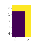
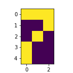
Let’s first try giving the network the following image of the digit 5:

(QUOTE (* * *
        * . .
        * * *
        . . *
        * * *))

It turns out like this:

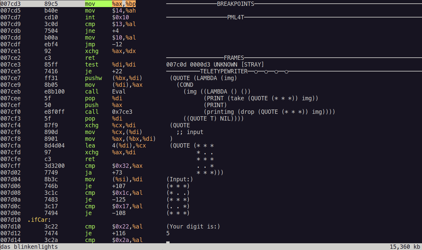
The network correctly predicts the digit shown in the image!

Although the original network was trained in an environment where 64-bit floating-point numbers were available, our system of 18-bit fixed-point numbers was also capable of running this network with the same parameters truncated to fit in 18 bits.

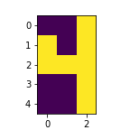
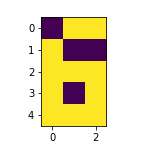
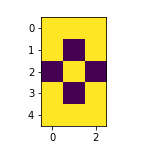
New Unseen Input with Noise

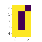
Now let’s try giving another digit:

(QUOTE (* * .
        . . *
        . * *
        * . .
        * * *))

Notice that this image is not apparent in the training set, or even in the test dataset. Therefore, the network has never seen this image before, and it is the very first time that it sees this image.

Can the network correctly predict the digit shown in this image? The results were as follows:

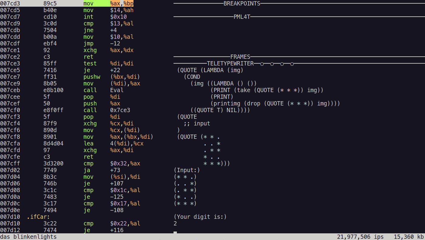
The network predicted the digit correctly!

Even for images that were never seen before, the neural network was able to learn how to interpret images of digits only by giving some examples of digit images. This is the magic of neural networks!

Therefore, in a way, we have taught a Lisp interpreter that runs on the IBM PC model 5150 what digits are, only by providing example pictures of digits in the process. Of course, the accumulation of knowledge through training the network was done on a modern computer, but that knowledge was handed on to a 512-byte program that is capable of running on vintage hardware.

Statistics

The training time for the neural network in TensorFlow was 6.5 seconds on a 6GB GTX 1060 GPU. The training was run on a 15-image dataset for 1000 epochs.

Here are the inference times of the neural network run in the emulators:

Emulator	Inference Time	Runtime Memory Usage
QEMU	4 seconds	64 kiB
Blinkenlights	2 minutes	64 kiB

The emulation was done on a 2.8 GHz Intel i7 CPU. When run on a 4.77 MHz IBM PC, I believe it should run 590 times slower than in QEMU, which is roughly 40 minutes.

The memory usage including the SectorLISP boot sector program, the S-expression stack for the entire Lisp program, and the RAM used for computing the neural network fits in 64 kiB of memory. This means that this program is capable of running on the original IBM 5150 PC.

Closing Remarks

It was very fun building a neural network from the bottom up using only first principles of symbolic manipulation. This is what it means for a programming language to be Turing-complete - it can basically do anything that any other modern computers are capable of.

As mentioned at the beginning of this post, Lisp was used as a language for creating advanced artificial intelligence after its birth in 1958. 60 years later in 2018, Yoshua Bengio, Geoffrey Hinton, and Yann LeCun received the Turing Award for establishing the foundations of modern Deep Learning. In a way, using a Turing-complete Lisp interpreter to implement neural networks revisits this history of computer science.

Credits

The neural network for SectorLISP and its fixed-point number system discussed in this blog post were implemented by Hikaru Ikuta. The SectorLISP project was first started by Justine Tunney and was created by the authors who have contributed to the project, and the authors credited in the original SectorLISP blog post. The i8086 emulator Blinkenlights was created by Justine Tunney. The neural network diagram was created using diagrams.net. The training and testing dataset, as well as the fully connected neural network model, were inspired by a blog post (in Japanese) written by Koichiro Mori (aidiary) from DeNA. The TensorFlow implementation of the model was referenced from the TensorFlow 2 quickstart for beginners entry from the TensorFlow documentation.